机器学习 | 计算分类算法的ROC和AUC曲线以随机森林为例

受试者工作特征（ROC）曲线和曲线下面积（AUC）是常用的分类算法评价指标，本文将讨论如何计算随机森林分类器的ROC 和 AUC。

ROC 和 AUC是量化二分类区分阳性和阴性类别能力的度量。ROC曲线是针对不同分类阈值的真阳性率（TPR）对假阳性率（FPR）的图。TPR是真阳性与阳性示例总数的比率，而FPR是假阳性与阴性示例总数的比率。AUC是ROC曲线下面积，范围为0.0至1.0，值越高表示分类器性能越好。

具体步骤

1.导入所需模块

from sklearn.ensemble import RandomForestClassifier 
from sklearn.metrics import roc_curve, roc_auc_score 
from sklearn.datasets import load_breast_cancer 
from sklearn.model_selection import train_test_split 
import matplotlib.pyplot as plt

这里我们导入所需的模块，包括分别来自sklearn.ensemble和sklearn.metrics模块的RandomForestClassifier和roc_curve函数。我们还从sklearn.datasets模块导入load_breast_cancer函数来加载乳腺癌数据集，并从sklearn.model_selection模块导入train_test_split函数来将数据集拆分为训练集和测试集。最后，我们从matplotlib库中导入pyplot模块来绘制ROC曲线。

2.加载并拆分数据集

加载数据集并分离特征和目标值，然后拆分训练和测试数据集。

df = load_breast_cancer(as_frame=True) 
df = df.frame 

x = df.drop('target',axis=1) 
y = df[['target']] 
# Split the dataset into training and test sets 
X_train, X_test, y_train, y_test = train_test_split(x, y, test_size=0.3)

3.训练随机森林分类器

# Train a Random Forest classifier 
rf = RandomForestClassifier(n_estimators=5, max_depth=2) 
rf.fit(X_train, y_train)

在这里，我们使用RandomForestClassifier函数训练一个随机森林分类器，其中包含5个估计量和最大深度2。我们使用拟合方法将分类器拟合到训练数据。

4.获取测试集的预测类概率

# Get predicted class probabilities for the test set 
y_pred_prob = rf.predict_proba(X_test)[:, 1] 

在这里，我们使用随机森林分类器的predict_proba方法来获得测试集的预测类概率。该方法返回一个形状数组（n_samples，n_classes），其中n_samples是测试集中的样本数，n_classes是问题中的类数。因为我们使用的是二元分类器，所以n_classes等于2，我们感兴趣的是正类的概率。 这是数组的第二列。因此，我们使用 [：,1] 索引来获得正类概率的一维数组。

5.计算不同分类阈值的假阳性率（FPR）和真阳性率（TPR）

# Compute the false positive rate (FPR) 
# and true positive rate (TPR) for different classification thresholds 
fpr, tpr, thresholds = roc_curve(y_test, y_pred_prob, pos_label=1)

在这里，我们使用sklearn.metrics模块中的roc_curve函数来计算不同分类阈值的假阳性率（FPR）和真阳性率（TPR）。该函数将测试集的真标签（y_test）和阳性类的预测类概率（y_pred_prob）作为输入。它返回三个数组：fpr，其包含不同阈值的FPR值; tpr，其包含不同阈值的TPR值;以及thresholds，其包含阈值。

6.计算ROC AUC评分

# Compute the ROC AUC score 
roc_auc = roc_auc_score(y_test, y_pred_prob) 
roc_auc

输出

0.9787264420331239

这里我们使用sklearn.metrics模块中的roc_auc_score函数来计算ROC AUC分数。该函数将测试集的真标签（y_test）和阳性类的预测类概率（y_pred_prob）作为输入。它返回表示ROC曲线下面积的标量值。

7.绘制ROC曲线

# Plot the ROC curve 
plt.plot(fpr, tpr, label='ROC curve (area = %0.2f)' % roc_auc) 
# roc curve for tpr = fpr 
plt.plot([0, 1], [0, 1], 'k--', label='Random classifier') 
plt.xlabel('False Positive Rate') 
plt.ylabel('True Positive Rate') 
plt.title('ROC Curve') 
plt.legend(loc="lower right") 
plt.show()

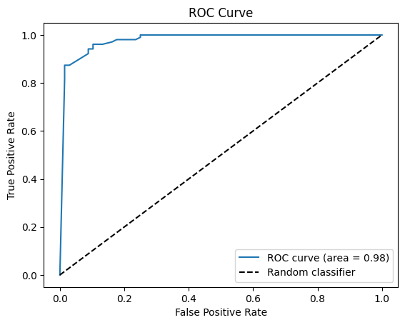
这里我们使用pyplot模块的plot函数来绘制ROC曲线。我们在x轴上传递FPR值，在y轴上传递TPR值。我们还将ROC AUC评分作为面积添加到图中。我们绘制虚线来表示随机分类器，其具有从（0，0）到（1，1）的直线的ROC曲线。我们为图添加轴标签和标题，以及显示ROC AUC得分和随机分类器线的图例。

说明：
ROC曲线是对于不同分类阈值，y轴上的真阳性率（TPR）对x轴上的假阳性率（FPR）的图。ROC曲线显示了分类器在不同阈值下区分阳性和阴性类别的能力。一个完美的分类器的TPR为1，FPR为0，对应于图的左上角。另一方面，随机分类器将具有从（0，0）到（1，1）的直线的ROC曲线，这是图中的虚线。ROC曲线越接近左上角，分类器的性能越好。

ROC曲线可用于选择分类器的最佳阈值，这取决于TPR和FPR之间的权衡。接近1的阈值将具有较低的FPR但较高的TPR，而接近0的阈值将具有较高的FPR但较低的TPR。

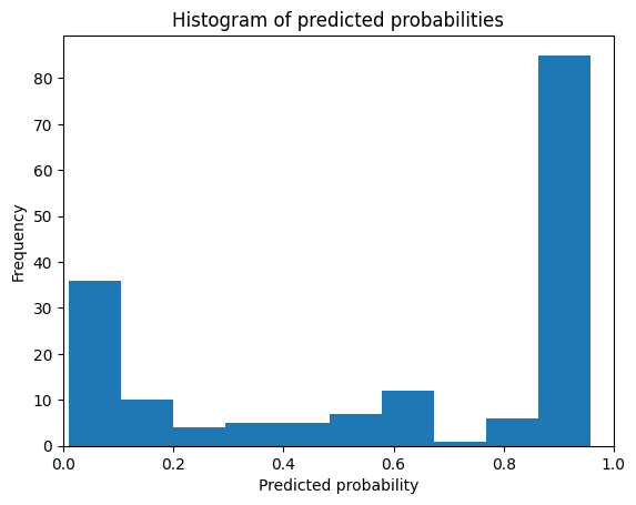
8.绘制预测类概率

# Plot the predicted class probabilities 
plt.hist(y_pred_prob, bins=10) 
plt.xlim(0, 1) 
plt.title('Histogram of predicted probabilities') 
plt.xlabel('Predicted probability of Setosa') 
plt.ylabel('Frequency') 
plt.show() 

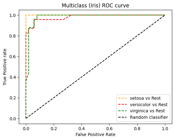
多分类的ROC曲线示例

这里使用sklearn.datasets的iris数据集，它有3个类。ROC曲线可用于二分类，因此，这里我们将使用来自sklearn.multiclass的OneVsRestClassifier和Random forest作为分类器，绘制ROC曲线。

from sklearn.ensemble import RandomForestClassifier 
from sklearn.metrics import roc_curve, roc_auc_score 
from sklearn.datasets import load_iris 
from sklearn.multiclass import OneVsRestClassifier 
from sklearn.model_selection import train_test_split 
import matplotlib.pyplot as plt 


# Load the iris dataset 
iris = load_iris() 

# Split the dataset into training and test sets 
X_train, X_test, y_train, y_test = train_test_split(iris.data, 
													iris.target, 
													test_size=0.5, 
													random_state=23) 

# Train a Random Forest classifier 
clf = OneVsRestClassifier(RandomForestClassifier()) 

# fit model 
clf.fit(X_train, y_train) 

# Get predicted class probabilities for the test set 
y_pred_prob = clf.predict_proba(X_test) 

# Compute the ROC AUC score 
roc_auc = roc_auc_score(y_test, y_pred_prob, multi_class='ovr') 
print('ROC AUC Score :',roc_auc) 

# roc curve for Multi classes 
colors = ['orange','red','green'] 
for i in range(len(iris.target_names)):	 
	fpr, tpr, thresh = roc_curve(y_test, y_pred_prob[:,i], pos_label=i) 
	plt.plot(fpr, tpr, linestyle='--',color=colors[i], label=iris.target_names[i]+' vs Rest') 
# roc curve for tpr = fpr 
plt.plot([0, 1], [0, 1], 'k--', label='Random classifier') 
plt.title('Multiclass (Iris) ROC curve') 
plt.xlabel('False Positive Rate') 
plt.ylabel('True Positive rate') 
plt.legend() 
plt.show()

输出

ROC AUC Score : 0.9795855072463767

总结

总之，计算随机森林分类器的ROC AUC分数在Python中是一个简单的过程。sklearn.metrics模块提供了计算ROC曲线、ROC AUC评分和PR曲线的函数。ROC曲线和PR曲线是评估二值分类器性能的有用工具，它们可以帮助基于不同评估指标之间的权衡来选择分类器的最佳阈值。

PR（precision-recall）曲线是二元分类问题的另一个评估指标。PR曲线是针对不同分类阈值的精确度（y轴）对召回率（x轴）的图。精确度被定义为真阳性的数量除以真阳性加假阳性的数量，而召回率被定义为真阳性的数量除以真阳性加假阴性的数量。PR曲线显示了分类器在最小化误报的同时预测阳性类别的能力。

与ROC曲线相比，PR曲线更适合不平衡数据集，其中阳性类别中的样本数量远小于阴性类别中的样本数量。当假阳性和假阴性的成本不同时，PR曲线也很有用，因为它可以帮助基于精确度-召回率权衡为分类器选择最佳阈值。

重要的是要注意，ROC AUC不应该是用于评估分类器性能的唯一度量。其他指标，如精确度、召回率和F1分数，也可能有用，具体取决于应用程序的具体要求。此外，重要的是要考虑数据中正面和负面示例的总体分布以及不平衡类对评估指标的潜在影响。