一文速学-XGBoost模型算法原理以及实现+Python项目实战_xgboost金融领域模型实战(1)

2401_84166376

于 2024-05-15 05:40:35 发布

阅读量978

点赞数 12

分类专栏：程序员文章标签：大数据面试学习

本文链接：https://blog.csdn.net/2401_84166376/article/details/138885515

版权

程序员专栏收录该内容

184 篇文章 0 订阅

订阅专栏

网上学习资料一大堆，但如果学到的知识不成体系，遇到问题时只是浅尝辄止，不再深入研究，那么很难做到真正的技术提升。

需要这份系统化资料的朋友，可以戳这里获取

一个人可以走的很快，但一群人才能走的更远！不论你是正从事IT行业的老鸟或是对IT行业感兴趣的新人，都欢迎加入我们的的圈子（技术交流、学习资源、职场吐槽、大厂内推、面试辅导），让我们一起学习成长！

对于决策树的例子大家可以参考我的上篇文章：

一文速学-GBDT模型算法原理以及实现+Python项目实战

这里不再复述，仅讲XGBoost改动，我们知道单独的使用GBDT模型，容易出现过拟合，在实际应用中往往使用 GBDT＋LR的方式做模型训练。一般情况下，我们的树模型越深越茂密那么复杂度越高，或者叶子节点值越大模型复杂度越高。

在XGBoost算法的实现中，是采用下式来衡量模型复杂度的：

$\Omega (f_{k})=\alpha T+\frac{1}{2}\lambda \sum_{j=1}{J}w_{j}{2}$

其中 $T$ 代表叶子节点个数， $\sum_{j=1}{J}w_{j}{2}$ :各个叶子节点值的求和， $\alpha ,\lambda$ ：超参数，控制惩罚程度。

那么我们将原目标函数的 $f_{t}(x_{i})$ 和 $\Omega (k_{t})$ 给取代掉：

$min\sum_{i=1}{n}[g_{j}w_{q(x_{i})}+\frac{1}{2}h_{i}w_{q(x_{i})}{2}]+\alpha T+\frac{1}{2}\lambda \sum_{j=1}^{J}\omega _{j}^{2}$

那么此时我们定义在叶子结点 $j$ 中的实例的集合为：

计算损失函数时是以样本索引来遍历的 $\sum_{i=1}^{n}$ 总共n个样本，计算所有叶子节点样本的损失可以为：

$\sum_{i\epsilon I_{j}}^{}g_{i}w_{j}$

所以此时目标函数就可以写为：

$\sum_{j=1}^{J}[(\sum_{i\epsilon I_{j}}^{}g_{i})w_{j}+(\frac{1}{2}\sum_{i\epsilon I_{j}}{}h_{i})w_{j}{2}]+\alpha T+\frac{1}{2}\lambda \sum_{j=1}{J}w_{j}{2}$

$=\sum_{j=1}^{J}[(\sum_{i\epsilon I_{j}}^{}g_{i})w_{j}+\frac{1}{2}(\sum_{i\epsilon I_{j}}h_{i}+\lambda )w_{j}^{2}]+\alpha T$

大家如果能看到这里已经差不多能将此目标函数推导出来了，但是这里我们还需要获得最优叶子结点的值，也就是最小值。此时我们需要将上述公式再度变换：

$G_{j}=\sum_{i\epsilon I_{j}}^{}g_{i}$

$H_{j}+\lambda =\sum_{i\epsilon I_{j}}^{}h_{i}+\lambda$

此时目函数就为 $G_{j}w_{j}+\frac{1}{2}(H_{j}+\lambda )w_{j}^{2}$ 是一个二次函数，对于二次函数这里补充一个大家或许真的的知识点，也就是得到这个函数的最小值。我们需要先求导去零得到极值点的x，再带入原方程。

那么对其求导很容易得到 $x=-\frac{G}{H}$ ,当 $x=-\frac{G}{H}$ 时对应方程的值为 $-\frac{1}{2}*\frac{G^{2}}{H}$ .

接着我们定义：

$G_{j}=\sum_{i\epsilon I_{j}}^{}g_{i}$
$H_{j}=\sum_{i\epsilon I_{j}}^{}h_{i}$

那么目标函数就为：

那么到这一步目标函数最优结构就确定了，但是针对于一棵树，模型的结构可能有很多种，此刻我们需要选择最优树结构，XGBoost算法采用的动态规划为贪心算法，去构建一颗最优的树。

不知道大家看到现在还有几个愿意看下去贪心算法构建最优树的，但是XGBoost算法的计算原理就是如此，要了解其计算过程这点是绕不过的，该学习了解的还是得下点功夫。

4.构建最优树(贪心算法)

贪心算法的模板下面给出：

确定问题的优化目标，即需要优化的指标。
将问题分解成若干个子问题，每个子问题都可以采取贪心策略求解。
对于每个子问题，定义一个局部最优解，然后利用贪心策略选择当前状态下的最优解，更新全局最优解。
对于更新后的全局最优解，判断是否满足问题的终止条件。如果满足，算法终止；如果不满足，继续执行步骤3。

而对于树模型的优劣程度我们是根据信息增益来判断的，也就是使用熵来进行评估不确定度，CART中使用的是基尼系数的概念。对于XGBoost算法来说我们比较 $Obj$ 的大小差距就可拟作信息增益 $Obj_{new}-Obj_{old}$ 。

我们是要获得最大信息增益，就需要遍历所以特征计算增益，选取增益大的进行切分构造树模型 $max=Obj_{new}-Obj_{old}$ 。

根据这个原理我们就可以构造一棵使目标函数最小的树模型，然后按照这个逻辑，一次构造K棵树，然后最终将所有的树加权就是我们最终的模型：

$f_{K}(x)=f_{K-1}(x)+f_{k}(x)=\sum_{k=1}^{K}f_{k}(x)$

讲到现在XGBoost已经讲完损失函数和分裂点选择两个核心的变动，还有另外四个改进，暂时先不作很深入的讲解，剪枝策略就详细介绍在RF算法中，正则化和提前停止策略我将会在下一篇详细讲述。下面进入实战实现环节。

三、XGBoost实战-贷款违约预测模型

或许大家觉得公式推导很繁琐，但是如果不做以上推导的话，无论是面试还是答辩无法证实你确实会使用XGBoost算法，而且面对XGBoost算法调优以及参数改进都是比较困难的。而且XGBoost一般直接使用自带的XGBoost库Python编程就好了，很少自行构造XGBoost树，大家可以参照我上篇文章GBDT流程一样构造XGBoost算法结构树。

对于贷款违约预测这个比较经典的课题，我们很容易拿到现成的数据，对于建模来讲，我们最缺的就是数据，而阿里天池提供了一份开源贷款违约数据，大家直接下载即可。

贷款违约预测

那么我们就开始实现逐步进行建模。

1.数据背景及描述

赛题以预测用户贷款是否违约为任务，数据集报名后可见并可下载，该数据来自某信贷平台的贷款记录，总数据量超过120w，包含47列变量信息，其中15列为匿名变量。为了保证比赛的公平性，将会从中抽取80万条作为训练集，20万条作为测试集A，20万条作为测试集B，同时会对employmentTitle、purpose、postCode和title等信息进行脱敏。

字段表

Field	Description
id	为贷款清单分配的唯一信用证标识
loanAmnt	贷款金额
term	贷款期限（year）
interestRate	贷款利率
installment	分期付款金额
grade	贷款等级
subGrade	贷款等级之子级
employmentTitle	就业职称
employmentLength	就业年限（年）
homeOwnership	借款人在登记时提供的房屋所有权状况
annualIncome	年收入
verificationStatus	验证状态
issueDate	贷款发放的月份
purpose	借款人在贷款申请时的贷款用途类别
postCode	借款人在贷款申请中提供的邮政编码的前3位数字
regionCode	地区编码
dti	债务收入比
delinquency_2years	借款人过去2年信用档案中逾期30天以上的违约事件数
ficoRangeLow	借款人在贷款发放时的fico所属的下限范围
ficoRangeHigh	借款人在贷款发放时的fico所属的上限范围
openAcc	借款人信用档案中未结信用额度的数量
pubRec	贬损公共记录的数量
pubRecBankruptcies	公开记录清除的数量
revolBal	信贷周转余额合计
revolUtil	循环额度利用率，或借款人使用的相对于所有可用循环信贷的信贷金额
totalAcc	借款人信用档案中当前的信用额度总数
initialListStatus	贷款的初始列表状态
applicationType	表明贷款是个人申请还是与两个共同借款人的联合申请
earliesCreditLine	借款人最早报告的信用额度开立的月份
title	借款人提供的贷款名称
policyCode	公开可用的策略_代码=1新产品不公开可用的策略_代码=2
n系列匿名特征	匿名特征n0-n14，为一些贷款人行为计数特征的处理

这里借用一下贷款违约预测学习笔记submarineas博主的图片

数据展示：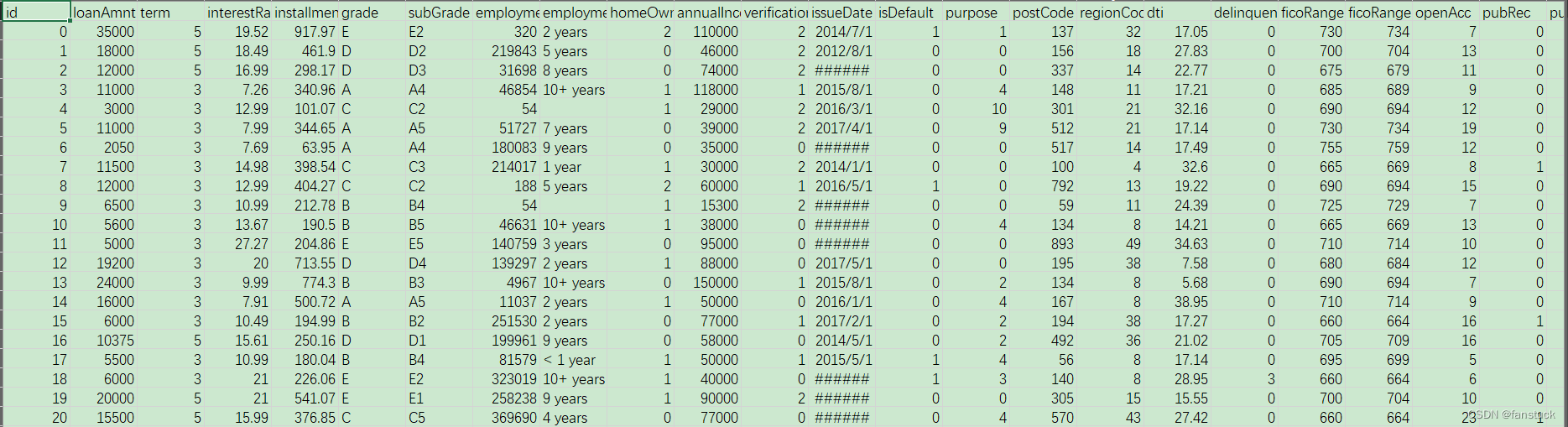

2.数据质量校验

使用pandas进行数据分析，也就是查看数据中的空缺值，重复值和异常值，以及相对应的数据描述。

import pandas as pd
df=pd.read_csv("train.csv")
test=pd.read_csv("testA.csv")

基本数据情况：

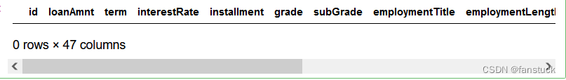
df.shape
(800000, 47)
test.shape
(200000, 46)

df.info()

<class 'pandas.core.frame.DataFrame'>
RangeIndex: 800000 entries, 0 to 799999
Data columns (total 47 columns):
 #   Column              Non-Null Count   Dtype  
---  ------              --------------   -----  
 0   id                  800000 non-null  int64  
 1   loanAmnt            800000 non-null  float64
 2   term                800000 non-null  int64  
 3   interestRate        800000 non-null  float64
 4   installment         800000 non-null  float64
 5   grade               800000 non-null  object 
 6   subGrade            800000 non-null  object 
 7   employmentTitle     799999 non-null  float64
 8   employmentLength    753201 non-null  object 
 9   homeOwnership       800000 non-null  int64  
 10  annualIncome        800000 non-null  float64
 11  verificationStatus  800000 non-null  int64  
 12  issueDate           800000 non-null  object 
 13  isDefault           800000 non-null  int64  
 14  purpose             800000 non-null  int64  
 15  postCode            799999 non-null  float64
 16  regionCode          800000 non-null  int64  
 17  dti                 799761 non-null  float64
 18  delinquency_2years  800000 non-null  float64
 19  ficoRangeLow        800000 non-null  float64
 20  ficoRangeHigh       800000 non-null  float64
 21  openAcc             800000 non-null  float64
 22  pubRec              800000 non-null  float64
 23  pubRecBankruptcies  799595 non-null  float64
 24  revolBal            800000 non-null  float64
 25  revolUtil           799469 non-null  float64
 26  totalAcc            800000 non-null  float64
 27  initialListStatus   800000 non-null  int64  
 28  applicationType     800000 non-null  int64  
 29  earliesCreditLine   800000 non-null  object 
 30  title               799999 non-null  float64
 31  policyCode          800000 non-null  float64
 32  n0                  759730 non-null  float64
 33  n1                  759730 non-null  float64
 34  n2                  759730 non-null  float64
 35  n3                  759730 non-null  float64
 36  n4                  766761 non-null  float64
 37  n5                  759730 non-null  float64
 38  n6                  759730 non-null  float64
 39  n7                  759730 non-null  float64
 40  n8                  759729 non-null  float64
 41  n9                  759730 non-null  float64
 42  n10                 766761 non-null  float64
 43  n11                 730248 non-null  float64
 44  n12                 759730 non-null  float64
 45  n13                 759730 non-null  float64
 46  n14                 759730 non-null  float64
dtypes: float64(33), int64(9), object(5)

查看重复值：

df[df.duplicated()==True]#打印重复值

缺失值统计

# nan可视化
missing = df.isnull().sum()/len(df)
missing = missing[missing > 0]
missing.sort_values(inplace=True)
missing.plot.bar()

异常值分析-MAD异常值识别法：

这里仅检测为数值的特征，对该方法不清楚的可以去看看我的另一篇文章一文速学(六)-数据分析之Pandas异常值检测及处理操作各类方法详解+代码展示-数据分析之Pandas异常值检测及处理操作各类方法详解+代码展示")：

3.特征类别处理

此时我们可以发现有五个特征为object特征，对于此特征我们需要进行特征转换，大家可以参考我的一文速学-特征数据类别分析与预处理方法详解+Python代码，处理定类特征。

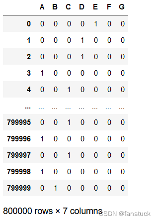
1.grade

该特征为贷款等级，总共有A,B,C,D,E,F,G七个等级，使用OneHot Encoding方法可行：

pd.get_dummies(df.grade,drop_first=False)

2.subGrade

该特征为贷款等级之子级，命名规则为贷款等级加上[1,2,3,4,5]这五个等级，这显然用OneHot Encoding方法就不行了，而且与上个grade方法存在信息冗余，因此可以将此特征与上个特征grade特征进行合并处理，通过适当加入一定的量纲即可。当然有更好的方法，我这里便于大家理解，采用一下方法：

df_grade=pd.get_dummies(df.grade,drop_first=False) 
def shine_convert(x):
    x=x*2
    return x/10 
se_subGrade=df.subGrade.str[1:].astype(int).apply(shine_convert)

for i in range(df_grade.shape[0]):
    data=df_grade.iloc[i,:]
    non_zero_index = data != 0
    data.loc[non_zero_index] += se_subGrade[i]
    print(data)

这里就实现了在定类数据上面再作等级的划分的条件。当然跑80w数据我这电脑以及够慢了，这里并没有跑完，大家可以去尝试一下。

4.XGBoost模型训练

数据处理的问题我这里不演示太多，毕竟主要是写XGBoost的运用，文章太长了也容易造成知识疲劳，这里我们就直接使用XGBoost算法，大家默认数据已经是处理好的就好了。这里详细讲一下XGBoost算法调参该如何调。

1.xgboost.get_config()

获取全局配置的当前值。
全局配置由可在全局范围中应用的参数集合组成。有关全局配置中支持的参数的完整列表：Global Configuration

import xgboost as xgb
xgb.get_config()

2.树的最大深度以及最小叶子节点样本权重

首先对这个值为树的最大深度以及最小叶子节点样本权重和这个组合进行调整。最大深度控制了树的结构，最小叶子节点样本权重这个参数用于避免过拟合。当它的值较大时，可以避免模型学习到局部的特殊样本。但是如果这个值过高，会导致欠拟合。

param_test1 = {'max_depth':range(3,10,2),'min_child_weight':range(2,7,2)}
 
gsearch1 = GridSearchCV(estimator =XGBR( learning_rate =0.1, n_estimators=140, max_depth=5,
                                         min_child_weight=1, gamma=0, subsample=0.8, colsample_bytree=0.8, objective= 'reg:linear',
                                         nthread=4, scale_pos_weight=1, seed=27),
                                         param_grid = param_test1, scoring='r2',n_jobs=4, cv=5)
gsearch1.fit(Xtrain,Ytrain)
gsearch1.best_params_, gsearch1.best_score_

3.gamma

再对参数 gamma 进行调整。在XGBoost 节点分裂时，只有分裂后损失函数的值下降了，才会分裂这个节点。gamma 指定了节点分裂所需的最小损失函数下降值。这个参数的大小决定了模型的保守程度。参数越高，模型越不保守。

param_test3 = {
 'gamma':[i/10.0 for i in range(0,5)]
}
gsearch3 = GridSearchCV(estimator = xgb.XGBClassifier( learning_rate =0.1, n_estimators=8, max_depth=8,
 min_child_weight=3, gamma=0, subsample=0.8, colsample_bytree=0.8,
 objective= 'binary:logistic', nthread=4, scale_pos_weight=1,seed=27), 
 param_grid = param_test3, scoring='roc_auc',iid=False, cv=5)
gsearch3.fit(X,y)
gsearch3.best_params_, gsearch3.best_score_

4.subsample 和 colsample_bytree

再对参数 subsample 和 colsample_bytree 进行调整。subsample 控制对于每棵树的随机采样的比例。减小这个参数的值，算法会更加保守，避免过拟合。但是，如果这个值设置得过小，它可能会导致欠拟合。colsample_bytree 用来控制每棵随机采样的列数的占比(每一列是一个特征)。

param_test4 = {
 'subsample':[i/100.0 for i in range(75,90,5)],
 'colsample_bytree':[i/100.0 for i in range(75,90,5)]
}
gsearch5 = GridSearchCV(estimator = xgb.XGBClassifier( learning_rate =0.1, n_estimators=8, max_depth=8,
 min_child_weight=3, gamma=0.4, subsample=0.8, colsample_bytree=0.8,
 objective= 'binary:logistic', nthread=4, scale_pos_weight=1,seed=27), 
 param_grid = param_test5, scoring='roc_auc',iid=False, cv=5)
gsearch5.fit(X_train,y_train)
gsearch5.best_params_, gsearch5.best_score_

5.正则项

控制模型的正则项，防止出现过拟合的现象。

param_test5 = {
 'reg_alpha':[1e-5, 1e-2, 0.1, 1, 100]
}
gsearch6 = GridSearchCV(estimator = xgb.XGBClassifier( learning_rate =0.1, n_estimators=8, max_depth=8,
 min_child_weight=3, gamma=0.2, subsample=0.85, colsample_bytree=0.85,
 objective= 'binary:logistic', nthread=4, scale_pos_weight=1,seed=27), 
 param_grid = param_test6, scoring='roc_auc',iid=False, cv=5)
gsearch6.fit(X_train,y_train)
gsearch6.best_params_, gsearch6.best_score_

6.学习速率

最后进行学习速率的调整，选择最优的学习速率最终确定适合的模型。

param_test6 = {
 'learning_rate':[0.01, 0.02, 0.1, 0.2]
}
gsearch6 = GridSearchCV(estimator = xgb.XGBClassifier( learning_rate =0.1, n_estimators=8, max_depth=8,
 min_child_weight=1, gamma=0.2, subsample=0.8, colsample_bytree=0.85,
 objective= 'binary:logistic', nthread=4, scale_pos_weight=1,seed=27), 
 param_grid = param_test6, scoring='roc_auc',iid=False, cv=5)
gsearch6.fit(X_train,y_train)
gsearch6.best_params_, gsearch6.best_score_

无参数XGBoost：

from sklearn.metrics import roc_auc_score
from sklearn.model_selection import train_test_split  
import xgboost as xgb
from sklearn.model_selection import KFold
from sklearn.metrics import confusion_matrix
import seaborn as sns
import matplotlib.pyplot as plt
train=pd.read_csv("df2.csv")
train=train.iloc[:10000,:] 
testA2=pd.read_csv("testA.csv")
    
# 划分特征变量与目标变量
X=train.drop(columns='isDefault')
Y=train['isDefault']
# 划分训练及测试集
x_train,x_test,y_train,y_test=train_test_split(X,Y,test_size=0.2,random_state=0)
# 模型训练
clf=xgb.XGBClassifier() 
result = []
mean_score = 0
labels=[0,1]
clf.fit(x_train,y_train)
y_pred=clf.predict_proba(x_test)[:,1]
def classify_convert(x):
    if x >0.5:
        return 1
    else:
        return 0
list_predict=[]
for i in y_pred:
    list_predict.append(classify_convert(i))

    
cm= confusion_matrix(y_test.values, list_predict)
sns.heatmap(cm,annot=True ,fmt="d",xticklabels=labels,yticklabels=labels)
print('验证集auc:{}'.format(roc_auc_score(y_test, y_pred)))
mean_score += roc_auc_score(y_test, y_pred)
plt.title('confusion matrix')  # 标题
plt.xlabel('Predict lable')  # x轴
plt.ylabel('True lable')  # y轴
plt.show()
# 模型评估
print('mean 验证集Auc:{}'.format(mean_score))
cat_pre=sum(result)  
from sklearn.metrics import f1_score
print('F1_socre:{}'.format(f1_score(y_test.values, list_predict, average='weighted')))
from sklearn.metrics import recall_score
print('Recall_score:{}'.format(recall_score(y_test.values, list_predict, average='weighted')))
from sklearn.metrics import precision_score
print('Percosopn:{}'.format(precision_score(y_test.values, list_predict, average='weighted')))

参数调整：

from sklearn.metrics import roc_auc_score
from sklearn.model_selection import train_test_split  
import xgboost as xgb
from sklearn.model_selection import KFold
from sklearn.metrics import confusion_matrix
import seaborn as sns
import matplotlib.pyplot as plt
train=pd.read_csv("df2.csv")
train=train.iloc[:10000,:] 
testA2=pd.read_csv("testA.csv")
    
# 划分特征变量与目标变量
X=train.drop(columns='isDefault')
Y=train['isDefault']
# 划分训练及测试集
x_train,x_test,y_train,y_test=train_test_split(X,Y,test_size=0.2,random_state=0)
# 模型训练
clf=xgb.XGBClassifier(eta=0.1,
                      n_estimators=8,
                      max_depth=8,
                      min_child_weight=2,
                      gamma=0.8,
                      subsample=0.85,
                      colsample_bytree=0.8
                     ) 
result = []
mean_score = 0
labels=[0,1]
clf.fit(x_train,y_train)


![img](https://img-blog.csdnimg.cn/img_convert/45ab602e75e5ebba3d1e1eff8db924a1.png)
![img](https://img-blog.csdnimg.cn/img_convert/93fcc76a9b6a554f8151ef6de6486c0e.png)

**网上学习资料一大堆，但如果学到的知识不成体系，遇到问题时只是浅尝辄止，不再深入研究，那么很难做到真正的技术提升。**

**[需要这份系统化资料的朋友，可以戳这里获取](https://bbs.csdn.net/topics/618545628)**


**一个人可以走的很快，但一群人才能走的更远！不论你是正从事IT行业的老鸟或是对IT行业感兴趣的新人，都欢迎加入我们的的圈子（技术交流、学习资源、职场吐槽、大厂内推、面试辅导），让我们一起学习成长！**

                min_child_weight=2,
                      gamma=0.8,
                      subsample=0.85,
                      colsample_bytree=0.8
                     ) 
result = []
mean_score = 0
labels=[0,1]
clf.fit(x_train,y_train)


[外链图片转存中...(img-grSeKiWF-1715722813032)]
[外链图片转存中...(img-6fZpRP6Q-1715722813032)]

**网上学习资料一大堆，但如果学到的知识不成体系，遇到问题时只是浅尝辄止，不再深入研究，那么很难做到真正的技术提升。**

**[需要这份系统化资料的朋友，可以戳这里获取](https://bbs.csdn.net/topics/618545628)**


**一个人可以走的很快，但一群人才能走的更远！不论你是正从事IT行业的老鸟或是对IT行业感兴趣的新人，都欢迎加入我们的的圈子（技术交流、学习资源、职场吐槽、大厂内推、面试辅导），让我们一起学习成长！**

2401_84166376

关注

12
点赞
踩
11

收藏

觉得还不错? 一键收藏
0
评论
一文速学-XGBoost模型算法原理以及实现+Python项目实战_xgboost金融领域模型实战(1)

这里不再复述，仅讲XGBoost改动，我们知道单独的使用GBDT模型，容易出现过拟合，在实际应用中往往使用 GBDT＋LR的方式做模型训练。一般情况下，我们的树模型越深越茂密那么复杂度越高，或者叶子节点值越大模型复杂度越高。在XGBoost算法的实现中，是采用下式来衡量模型复杂度的：其中代表叶子节点个数，:各个叶子节点值的求和，：超参数，控制惩罚程度。那么我们将原目标函数的和给取代掉：那么此时我们定义在叶子结点中的实例的集合为：计算损失函数时是以样本索引来遍历的。
复制链接

扫一扫