


据相关媒体报道,2023 年考研可以称得上是“最难”的一年,全国研究生报 考人数突破新高达到 474 万人、部分考研学生感染新冠带病赴考、保研名额增多 挤压考研录取名额等因素都导致了2023 年考研上岸难度加大。不少同学参加完 2023 年考研直呼:今年考研也太难了!
从客观的角度来说,2023 年考研确实不简单,考研难度甚至超过了之前的 任何一年。报考人数突破新高,保研率持续上涨,录取率降低。不少 985 高校保 研率都已经突破了 50%,考取 985 高校的考生竞争非常激烈,录取的可能进一步 降低。从数据来看,2023 年考研上岸的难度比往年更大。根据不完全统计,2023 年考研录取率将低于 20% ,将有超过 300 万考生落榜。
基于以上背景,请你们的团队收集相关数据,研究解决以下问题:
5.2问题 : 预测未来 3 年考研难度的变化,基于你们的研究给报考2024年研究生的广大考生提几条建议。
为了探讨未来三年考研的难度变化:我们这里采用时间序列的ARIMA模型来求解,ARIMA模型作为时间序列分析的常见方法之一,主要 是从时序数据自相关的角度反映其本身的发展规律,它本身十分简单,只与内生变量有关而无须借助外部变量.
5.2.1模型介绍和求解
5.2.1.1模型用途
自回归移动平均模型(Autoregressive Integrated Moving Average Model,ARIMA)是由 Box 和 Jenkins 在 20 世纪 70 年代初提出的时间序列检测方法,又称为Box-jenkins模型。它在统计学和计量经济学等多种学科当中都有所应 用,是最常见的一种用于进行时间序列预测的方法。
其实,ARIMA模型是AR,I和MA多个模型的具体表现形式,具体取决于,是否是否对序列差分,是否由数据本身或本身差分项的回归构成,是否由随机序列的回归构成。
5.2.1.2自回归模型AR
p 阶自回归模型的公式定义为:
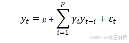
值得一提的是最后一项为白噪声项,满足总和为0,
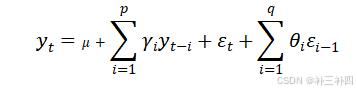
5.2.1.3衍生至ARIMA模型
由于0阶或1阶的AR模型稳定性不足,我们通过差分(I)的方式得到更进一步的模型,并由于AR模型中yt-1受白噪声εt-1的影响而使εt-1也对yt产生影响,因此我们这里引入滑动平均模型(MA),最终得到的就是ARIMA模型
为体现时序数据中,相邻观测点的相关程度,我们采用的是正相关函数:
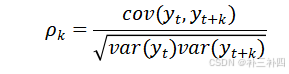
得到自相关系数ACF。
偏自相关系数(PACF)是随机变量去除中间k-1个值影响后衡量yt和yt-k之间的相关性,这里公式较为复杂,难以通过封闭公式直接给出。
5.2.1.3参数d的介绍和确定方法
在ARIMA模型中,参数 d表示差分的次数,用于将非平稳时间序列转换为平稳时间序列。具体来说,d是使时间序列成为平稳序列所需的差分阶数。通过差分,可以去除时间序列中的趋势成分,使其满足平稳性的要求,从而可以应用ARMA模型进行建模。
| 模型 | ACF | PACF |
| AR(p) | 拖尾 | p阶后截尾 |
| MA(q) | q阶后截尾 | 拖尾 |
| ARMA(p,q) | q阶后拖尾 | p阶后拖尾 |
参数p,q和模型的确定条件
给出差分操作的代码
def difference_series(series, d=1):

    # 进行差分操作

    for _ in range(d):

        series = series.diff().dropna()

return series
5.2.2数据准备
由于上述数据过少,我们使用python中的acf和pacf函数时,滞后值只能设置为一,因此,我们删除掉仅有三年数据的保研公示人数来继续分析
|
| 报考人数 | 录取率 | A类平均考研成绩 |
| 2023 | 474 | 24.23% | 315.77 |
| 2022 | 457 | 24.15% | 320.46 |
| 2021 | 377 | 27.87% | 310.46 |
| 2020 | 341 | 29.05% | 310.77 |
import numpy as np
import pandas as pd
import matplotlib.pyplot as plt
from statsmodels.tsa.stattools import acf, pacf
# 设置支持中文的字体
plt.rcParams['font.sans-serif'] = ['SimHei'] # 用黑体显示中文
plt.rcParams['axes.unicode_minus'] = False # 正确显示负号
# 数据准备
data = {
'年份': [2020, 2021, 2022, 2023],
'报考人数': [341, 377, 457, 474],
'录取率': [29.05, 27.87, 24.15, 24.23],
'A类平均考研成绩': [310.77, 310.46, 320.46, 315.77]
}
df = pd.DataFrame(data)
df.set_index('年份', inplace=True)
# 选择一个时间序列列,例如 '报考人数'
ts = df['报考人数']
# 计算ACF和PACF值
acf_values = acf(ts, nlags=2)
pacf_values = pacf(ts, nlags=2)
# 计算置信区间
conf_int = 1.96 / np.sqrt(len(ts))
# 绘制ACF柱状图
plt.figure(figsize=(12, 6))
plt.bar(range(len(acf_values)), acf_values, color='blue', alpha=0.7)
plt.axhline(y=0, color='black', linestyle='--')
plt.axhline(y=-conf_int, color='red', linestyle='--', label='95% 置信区间')
plt.axhline(y=conf_int, color='red', linestyle='--')
plt.title('ACF图')
plt.xlabel('滞后期')
plt.ylabel('自相关系数')
plt.xticks(range(len(acf_values)), labels=range(len(acf_values)))
plt.legend()
plt.show()
# 绘制PACF柱状图
plt.figure(figsize=(12, 6))
plt.bar(range(len(pacf_values)), pacf_values, color='blue', alpha=0.7)
plt.axhline(y=0, color='black', linestyle='--')
plt.axhline(y=-conf_int, color='red', linestyle='--', label='95% 置信区间')
plt.axhline(y=conf_int, color='red', linestyle='--')
plt.title('PACF图')
plt.xlabel('滞后期')
plt.ylabel('偏自相关系数')
plt.xticks(range(len(pacf_values)), labels=range(len(pacf_values)))
plt.legend()
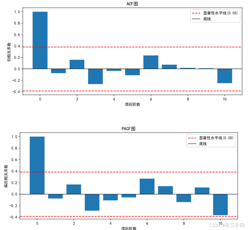
plt.show()对其进行ADF检验,看起来,此时报考人数的ACF和PACF图都不为拖尾和截尾
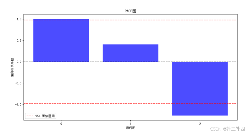
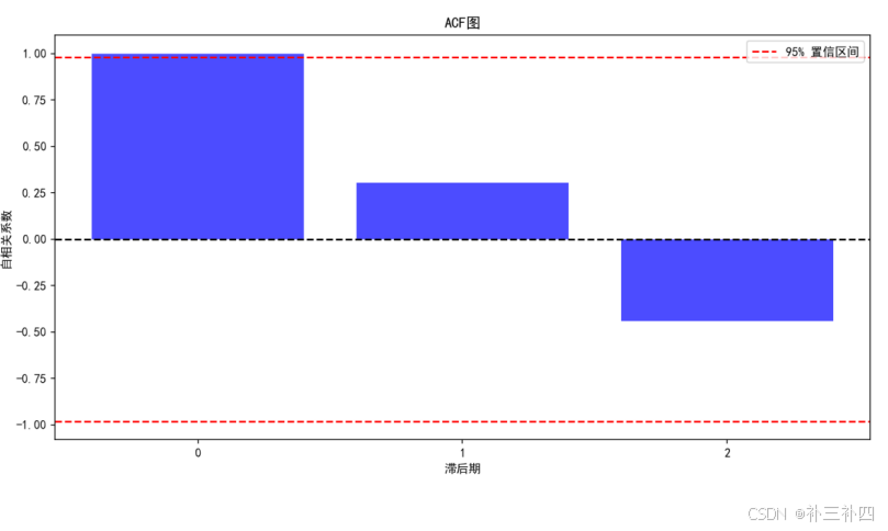
当然,也可以通过ADF检验来判断是否进一步差分
# 进行ADF检验
def adf_test(series):

    result = adfuller(series)

    print(f'ADF Statistic: {result[0]}')

    print(f'p-value: {result[1]}')

    print(f'Critical Values: {result[4]}')

return result[1]  # 返回p-value
5.2.3平稳性分析与pq的确定:
但是由于数据量过小,不能继续对其进行差分后用python分析
我只好把考研平均成绩也删掉,仅用报考人数和录取率进行分析
| 年份 | 报名人数(万) | 录取率(%) |
| 1997 | 24.20 | 21.08 |
| 1998 | 27.40 | 21.17 |
| 1999 | 31.90 | 20.38 |
| 2000 | 39.20 | 21.69 |
| 2001 | 46.00 | 24.02 |
| 2002 | 62.40 | 31.25 |
| 2003 | 79.70 | 33.88 |
| 2004 | 94.50 | 34.92 |
| 2005 | 117.20 | 27.72 |
| 2006 | 127.12 | 31.69 |
| 2007 | 128.20 | 28.40 |
| 2008 | 120.00 | 32.50 |
| 2009 | 124.60 | 33.31 |
| 2010 | 140.00 | 33.71 |
| 2011 | 151.10 | 32.76 |
| 2012 | 165.60 | 31.48 |
| 2013 | 176.00 | 30.73 |
| 2014 | 172.00 | 31.90 |
| 2015 | 164.90 | 34.58 |
| 2016 | 177.00 | 33.32 |
| 2017 | 201.00 | 35.82 |
| 2018 | 238.00 | 32.02 |
| 2019 | 290.00 | 27.93 |
| 2020 | 341.00 | 29.05 |
| 2021 | 377.00 | 27.87 |
| 2022 | 457.00 | 24.15 |
| 2023 | 474.00 | 24.23 |
import numpy as np

import pandas as pd

import matplotlib.pyplot as plt

from statsmodels.tsa.stattools import acf, pacf


# 设置支持中文的字体

plt.rcParams['font.sans-serif'] = ['SimHei']  # 用黑体显示中文

plt.rcParams['axes.unicode_minus'] = False  # 正确显示负号


# 数据准备

data = {

    '年份': list(range(1997, 2024)),

    '报考人数': [24.20, 27.40, 31.90, 39.20, 46.00, 62.40, 79.70, 94.50, 117.20, 127.12, 128.20, 120.00, 124.60, 140.00, 151.10, 165.60, 176.00, 172.00, 164.90, 177.00, 201.00, 238.00, 290.00, 341.00, 377.00, 457.00, 474.00],

    '录取率': [21.08, 21.17, 20.38, 21.69, 24.02, 31.25, 33.88, 34.92, 27.72, 31.69, 28.40, 32.50, 33.31, 33.71, 32.76, 31.48, 30.73, 31.90, 34.58, 33.32, 35.82, 32.02, 27.93, 29.05, 27.87, 24.15, 24.23]

}

df = pd.DataFrame(data)

df.set_index('年份', inplace=True)


# 选择一个时间序列列,例如 '报考人数'

ts = df['报考人数']


# 计算ACF和PACF值

acf_values = acf(ts, nlags=9)

pacf_values = pacf(ts, nlags=13)


# 计算置信区间

conf_int = 1.96 / np.sqrt(len(ts))


# 绘制ACF柱状图

plt.figure(figsize=(12, 6))

plt.bar(range(len(acf_values)), acf_values, color='blue', alpha=0.7)

plt.axhline(y=0, color='black', linestyle='--')

plt.axhline(y=-conf_int, color='red', linestyle='--', label='95% 置信区间')

plt.axhline(y=conf_int, color='red', linestyle='--')

plt.title('ACF图')

plt.xlabel('滞后期')

plt.ylabel('自相关系数')

plt.xticks(range(len(acf_values)), labels=range(len(acf_values)))

plt.legend()

plt.show()


# 绘制PACF柱状图

plt.figure(figsize=(12, 6))

plt.bar(range(len(pacf_values)), pacf_values, color='blue', alpha=0.7)

plt.axhline(y=0, color='black', linestyle='--')

plt.axhline(y=-conf_int, color='red', linestyle='--', label='95% 置信区间')

plt.axhline(y=conf_int, color='red', linestyle='--')

plt.title('PACF图')

plt.xlabel('滞后期')

plt.ylabel('偏自相关系数')

plt.xticks(range(len(pacf_values)), labels=range(len(pacf_values)))

plt.legend()

plt.show()
看上去没有经过差分的数据就有了十分优良的拟合效果:
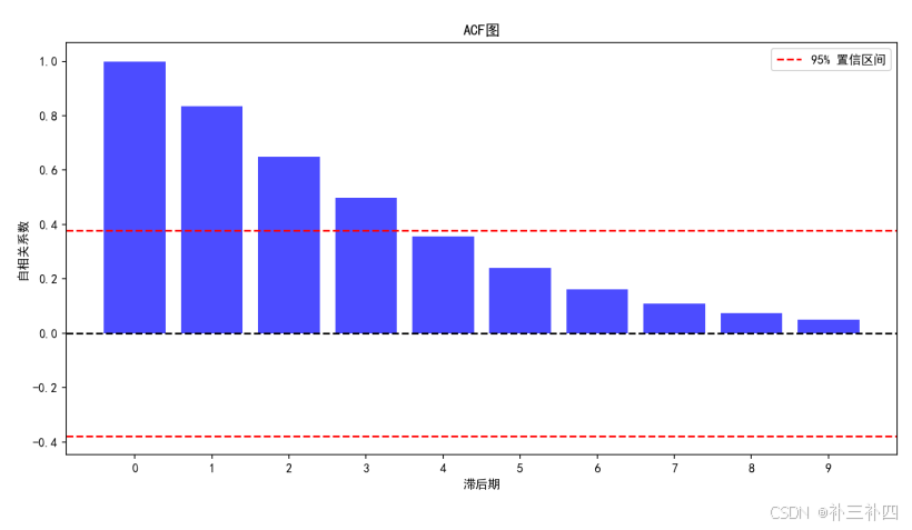
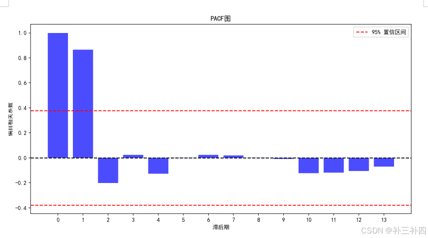
但仍应进行ADF检验:
ADF Statistic: 1.439546
p-value: 0.997287
Critical Values:
1%: -3.770
5%: -3.005
10%: -2.643
不能拒绝原假设,时间序列是非平稳的
说明ACF图实际上在后期不断减小而并非平稳
对报考人数进一步进行差分:
import numpy as np

import pandas as pd

import matplotlib.pyplot as plt

from statsmodels.tsa.stattools import adfuller, acf, pacf

from statsmodels.tsa.arima.model import ARIMA

from sklearn.metrics import mean_absolute_error, mean_squared_error

import pandas as pd

# 数据准备

data = {

    '年份': pd.date_range(start='1997-01-01',end='2023-01-01',freq='YS'),

    '报考人数': [24.20, 27.40, 31.90, 39.20, 46.00, 62.40, 79.70, 94.50, 117.20, 127.12, 128.20, 120.00, 124.60, 140.00, 151.10, 165.60, 176.00, 172.00, 164.90, 177.00, 201.00, 238.00, 290.00, 341.00, 377.00, 457.00, 474.00],

    '录取率': [21.08, 21.17, 20.38, 21.69, 24.02, 31.25, 33.88, 34.92, 27.72, 31.69, 28.40, 32.50, 33.31, 33.71, 32.76, 31.48, 30.73, 31.90, 34.58, 33.32, 35.82, 32.02, 27.93, 29.05, 27.87, 24.15, 24.23]

}

df = pd.DataFrame(data)

df.set_index('年份', inplace=True)

# 选择一个时间序列列,例如 '报考人数'

ts = df['报考人数']

import pandas as pd

# 创建DataFrame

df = pd.DataFrame(data)

# 将 '年份' 列转换为日期时间格式,并设置为索引

# 确保 '年份' 列存在于DataFrame中

if '年份' in df.columns:

    df['年份'] = pd.to_datetime(df['年份'].astype(str), format='%Y-%m-%d')

    df.set_index('年份', inplace=True)

    # 如果数据是年度数据,可以设置索引频率为年度,例如 'AS' 表示年初频率

    df.index.freq = 'YS'

else:

    print("DataFrame中不存在 '年份' 列。")

# 继续后续操作...

# 设置支持中文的字体

plt.rcParams['font.sans-serif'] = ['SimHei']  # 用黑体显示中文

plt.rcParams['axes.unicode_minus'] = False  # 正确显示负号

# 进行ADF检验

result = adfuller(ts, autolag='AIC')

print('ADF Statistic: %f' % result[0])

print('p-value: %f' % result[1])

print('Critical Values:')

for key, value in result[4].items():

    print('\t%s: %.3f' % (key, value))

# 判断时间序列是否平稳

if result[1] < 0.05:

    print('时间序列是平稳的')

else:

    print('时间序列是非平稳的')

# 如果时间序列是非平稳的,进行一阶差分

if result[1] >= 0.05:

    ts_diff = ts.diff().dropna()

    result_diff = adfuller(ts_diff, autolag='AIC')

    print('一阶差分后的ADF Statistic: %f' % result_diff[0])

    print('一阶差分后的p-value: %f' % result_diff[1])

    print('一阶差分后的Critical Values:')

    for key, value in result_diff[4].items():

        print('\t%s: %.3f' % (key, value))

    if result_diff[1] < 0.05:

        print('一阶差分后时间序列是平稳的')

        ts = ts_diff

        d = 1

    else:

        print('一阶差分后时间序列仍非平稳,需要进一步处理')

        d = 2

else:

d = 0

ADF Statistic: 1.439546

p-value: 0.997287

Critical Values:

1%: -3.770

5%: -3.005

10%: -2.643

时间序列是非平稳的

一阶差分后的ADF Statistic: -1.022306

一阶差分后的p-value: 0.745042

一阶差分后的Critical Values:

1%: -3.738

5%: -2.992

10%: -2.636

一阶差分后时间序列仍非平稳,需要进一步处理

经检验,仍非平稳

因此我们还要继续进行差分

import numpy as np

import pandas as pd

import matplotlib.pyplot as plt

from statsmodels.tsa.stattools import adfuller, acf, pacf

from statsmodels.tsa.arima.model import ARIMA

from sklearn.metrics import mean_absolute_error, mean_squared_error


# 设置支持中文的字体

plt.rcParams['font.sans-serif'] = ['SimHei']  # 用黑体显示中文

plt.rcParams['axes.unicode_minus'] = False  # 正确显示负号


# 数据准备

data = {

    '年份': pd.date_range(start='1997-01-01', end='2023-01-01', freq='YS'),

    '报考人数': [24.20, 27.40, 31.90, 39.20, 46.00, 62.40, 79.70, 94.50, 117.20, 127.12, 128.20, 120.00, 124.60, 140.00, 151.10, 165.60, 176.00, 172.00, 164.90, 177.00, 201.00, 238.00, 290.00, 341.00, 377.00, 457.00, 474.00],

    '录取率': [21.08, 21.17, 20.38, 21.69, 24.02, 31.25, 33.88, 34.92, 27.72, 31.69, 28.40, 32.50, 33.31, 33.71, 32.76, 31.48, 30.73, 31.90, 34.58, 33.32, 35.82, 32.02, 27.93, 29.05, 27.87, 24.15, 24.23]

}

df = pd.DataFrame(data)

df.set_index('年份', inplace=True)


# 选择一个时间序列列,例如 '报考人数'

ts = df['报考人数']


# 进行ADF检验

result = adfuller(ts, autolag='AIC')

print('ADF Statistic: %f' % result[0])

print('p-value: %f' % result[1])

print('Critical Values:')

for key, value in result[4].items():

    print('\t%s: %.3f' % (key, value))


# 判断时间序列是否平稳

if result[1] < 0.05:

    print('时间序列是平稳的')

else:

    print('时间序列是非平稳的')


# 如果时间序列是非平稳的,进行一阶差分

if result[1] >= 0.05:

    ts_diff = ts.diff().dropna()

    result_diff = adfuller(ts_diff, autolag='AIC')

    print('一阶差分后的ADF Statistic: %f' % result_diff[0])

    print('一阶差分后的p-value: %f' % result_diff[1])

    print('一阶差分后的Critical Values:')

    for key, value in result_diff[4].items():

        print('\t%s: %.3f' % (key, value))


    if result_diff[1] >= 0.05:

        print('一阶差分后时间序列仍非平稳,进行二阶差分')

        ts_diff2 = ts_diff.diff().dropna()

        result_diff2 = adfuller(ts_diff2, autolag='AIC')

        print('二阶差分后的ADF Statistic: %f' % result_diff2[0])

        print('二阶差分后的p-value: %f' % result_diff2[1])

        print('二阶差分后的Critical Values:')

        for key, value in result_diff2[4].items():

            print('\t%s: %.3f' % (key, value))


        if result_diff2[1] < 0.05:

            print('二阶差分后时间序列是平稳的')

            ts = ts_diff2

            d = 2

        else:

            print('二阶差分后时间序列仍非平稳,需要进一步处理')

            d = 3

    else:

        print('一阶差分后时间序列是平稳的')

        ts = ts_diff

        d = 1

else:

d = 0
最终得到二阶差分是平稳的:
ADF Statistic: 1.439546
p-value: 0.997287
Critical Values:
1%: -3.770
5%: -3.005
10%: -2.643
时间序列是非平稳的
一阶差分后的ADF Statistic: -1.022306
一阶差分后的p-value: 0.745042
一阶差分后的Critical Values:
1%: -3.738
5%: -2.992
10%: -2.636
一阶差分后时间序列仍非平稳,进行二阶差分
二阶差分后的ADF Statistic: -6.516956
二阶差分后的p-value: 0.000000
二阶差分后的Critical Values:
1%: -3.738
5%: -2.992
10%: -2.636
二阶差分后时间序列是平稳的
再绘制acf和pacf图:
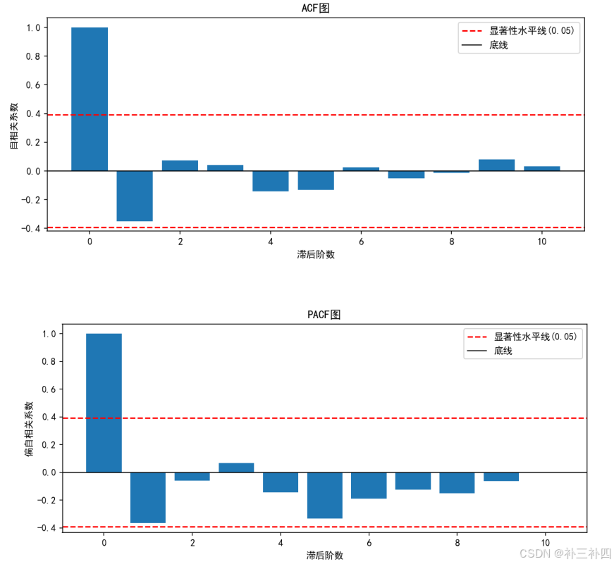
然后我们再对后三年的数据进行预测:
from statsmodels.tsa.arima.model import ARIMA

# 报考人数数据

data = [24.20, 27.40, 31.90, 39.20, 46.00, 62.40, 79.70, 94.50, 117.20, 127.12, 128.20, 120.00, 124.60, 140.00, 151.10, 165.60, 176.00, 172.00, 164.90, 177.00, 201.00, 238.00, 290.00, 341.00, 377.00, 457.00, 474.00]

# 拟合ARIMA模型,手动设置初始参数

model = ARIMA(data, order=(1, 2, 1))

result = model.fit()  # 对模型进行拟合

# 打印模型摘要

print(result.summary())

# 进行预测

forecast = result.forecast(steps=3)  # 预测未来3年的报考人数

# 打印预测结果

print("未来3年的报考人数预测:")

print(forecast)

得到结果:

[532.93875644 560.56474811 611.56981252]
同理,对录取率进行ADF检验,得到一阶差分后的时间序列是平稳的。
并进行结果预测:
[24.02384475 24.19244881 24.05455599]
为探究后三年的高考难度分数,我们需要将上一篇blog中的基于层次分析法赋权的TOPSIS法引用过来:
由于参加考研的人数超过以前,不能用原基准下的max_admission_rate
并且要对于权重[0.0694, 0.4893]重新进行归一化处理,相比原来有所改进的点是我们对数据的正向化直接采取1-录取率:
import numpy as np

# 创建矩阵(去掉年份列)

data_matrix = np.array([

    [24.20, 0.2108],

    [27.40, 0.2117],

    [31.90, 0.2038],

    [39.20, 0.2169],

    [46.00, 0.2402],

    [62.40, 0.3125],

    [79.70, 0.3388],

    [94.50, 0.3492],

    [117.20, 0.2772],

    [127.12, 0.3169],

    [128.20, 0.2840],

    [120.00, 0.3250],

    [124.60, 0.3331],

    [140.00, 0.3371],

    [151.10, 0.3276],

    [165.60, 0.3148],

    [176.00, 0.3073],

    [172.00, 0.3190],

    [164.90, 0.3458],

    [177.00, 0.3332],

    [201.00, 0.3582],

    [238.00, 0.3202],

    [290.00, 0.2793],

    [341.00, 0.2905],

    [377.00, 0.2787],

    [457.00, 0.2415],

    [474.00, 0.2423],

    [532.93, 0.2402],

    [560.56, 0.2419],

    [611.57, 0.2405]

])


# 对录取率进行正向化处理 (1 - 录取率)

data_matrix[:, 1] = 1 - data_matrix[:, 1]

print("正向化处理后的矩阵:")

print(data_matrix)


# 计算每一列元素的平方和

column_sums_of_squares = np.sum(data_matrix**2, axis=0)

print("每一列元素的平方和:")

print(column_sums_of_squares)


# 标准化:对每一列元素除以该列的平方和的平方根

data_matrix = data_matrix / np.sqrt(column_sums_of_squares)

print("标准化处理后的矩阵:")

print(data_matrix)


# 赋权

weights = np.array([0.0694, 0.4893])

normalized_weights = weights / np.sum(weights)

weighted_matrix = data_matrix * normalized_weights

print("赋权后的矩阵:")

print(weighted_matrix)

# 计算正理想解和负理想解

positive_ideal_solution = np.max(weighted_matrix, axis=0)

negative_ideal_solution = np.min(weighted_matrix, axis=0)

print("正理想解:", positive_ideal_solution)

print("负理想解:", negative_ideal_solution)

# 计算2024、2025、2026年与正理想解和负理想解的距离

distances_to_positive_ideal = np.linalg.norm(weighted_matrix[-3:, :] - positive_ideal_solution, axis=1)

distances_to_negative_ideal = np.linalg.norm(weighted_matrix[-3:, :] - negative_ideal_solution, axis=1)

print("到正理想解的距离:", distances_to_positive_ideal)

print("到负理想解的距离:", distances_to_negative_ideal)

# 计算2024、2025、2026年的相对接近度

relative_closeness = distances_to_negative_ideal / (distances_to_positive_ideal + distances_to_negative_ideal)

print("相对接近度(分数):", relative_closeness)

# 输出2024、2025、2026年的高考难度分数

for year, score in zip([2024, 2025, 2026], relative_closeness):

print(f"{year}年的高考难度分数: {score}")
最后得到:
2024年的高考难度分数: 0.8277752773131622
2025年的高考难度分数: 0.8457816098873717
2026年的高考难度分数: 0.8728741764602923
5.3模型的缺陷:
1.arima模型本身对大量数据的依赖与数据缺失之间的矛盾会导致模型精准度降低
2.TOPSIS法由于受新加入的值可能会对原本的最大值造成影响,导致数值难以长期稳定,不适合用于求解时间序列下的分数。
参考文献:闫祥祥.使用ARIMA模型预测公园绿地面积[J].计算机科学,2020,47(S2):531-534,556.


 9407
9407

 被折叠的 条评论
为什么被折叠?
被折叠的 条评论
为什么被折叠?
 到【灌水乐园】发言


