Wasserstein GAN

概要

Wasserstein GAN(简称WGAN)提出了一种Wasserstein损失，为了解决传统GAN训练中存在的一些问题，如训练不稳定和模式崩溃等。

Wasserstein距离

Wasserstein距离的定义如下：
$$W(P_r,P_g)=\underset{||f|{|}_L\le 1}{\sup }{\mathbb{E}}_{x\sim P_r}[f(x)]-{\mathbb{E}}_{\tilde{x}\sim P_g}[f(\tilde{x})]$$

判别器$D(x)$对应$f(x)$，这个公式的包括两个部分，首先是两个分布的距离要大，第二是对判别器有一个约束。$||f|{|}_L\le 1$意味着$f$必须是1-Lipschitz函数（定义如下）。

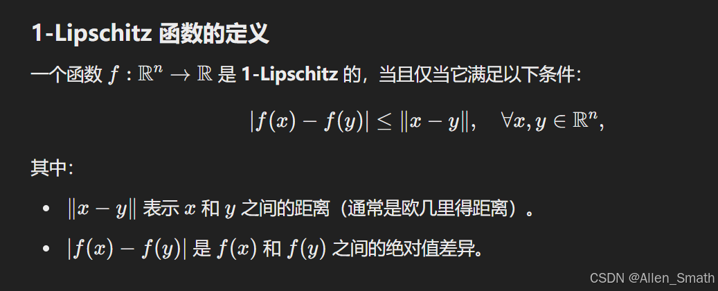
sup表示上确界，这里表示在所有1-Lipchitz函数$f$上取上确界。在WGAN中，1-Lipchitz性是通过梯度惩罚实现的。

WGAN判别器损失函数

从上一节可以看出，判别器主要是为了能准确识别出源域和目标域，也就是最大化二者的Wasserstein距离，即
$$\underset{D}{\max }{\mathbb{E}}_{x\sim P_r}[f(x)]-{\mathbb{E}}_{\tilde{x}\sim P_g}[f(\tilde{x})]$$
其中，$P_r$是真实分布，$P_g$是生成器的分布，在训练过程中，将最大化目标转化味最小化该目标的负值：
$$L_D=-{\mathbb{E}}_{x\sim P_r}[f(x)]+{\mathbb{E}}_{\tilde{x}\sim P_g}[f(\tilde{x})]$$
真实样本的得分应该尽可能高，生成样本的得分应尽可能低，最大化二者分数的差异。加入梯度惩罚后：
$$L_D=-{\mathbb{E}}_{x\sim P_r}[f(x)]+{\mathbb{E}}_{\tilde{x}\sim P_g}[f(\tilde{x})]+\lambda \cdot gradientpenalty$$
其中，梯度惩罚的计算为：
$$gradientpenalty={\mathbb{E}}_{\hat{x}\sim P_{interp}}(||{\nabla }_{\hat{x}}D(\hat{x})|{|}_2-1{)}^2$$
$P_{interp}$是在真实和生成样本之间随机插值得到的分布。

梯度惩罚损失项代码：

def compute_gradient_penalty(D,real_samples, fake_samples):
	#D是判别器，real_smaple是真实样本，fake_sample是虚假样本，也就是生成样本
    alpha = torch.cuda.FloatTensor(np.random.random((real_samples.size(0),1,1)))
    #这里的alpha是初始化插值权重
    interpolates = (alpha * real_samples +(1-alpha)*fake_samples).requires_grad_(True)
	#根据权重、真实样本和生成样本计算插值样本，require_grad 这里让张量可以计算梯度
    d_interpolates = D(interpolates)
    fake = Variable(torch.cuda.FloatTensor(np.ones(d_interpolates.shape)), requires_grad=False)
    gradients = autograd.grad(outputs=d_interpolates,
                              inputs=interpolates,
                              grad_outputs=fake,
                              create_graph=True, retain_graph=True, only_inputs=True)[0]
	#outputs是判别器输出，inputs是插值样本，grad_outputs使用单位张量作为梯度的权重
    gradients = gradients.view(gradients.size(0), -1)
    #将梯度展平成一维
    gradient_penalty = ((gradients.norm(2, dim=1) - 1) ** 2).mean()
    #计算二范数
    return gradient_penalty

WGAN生成器损失函数

生成器的任务就是使Wasserstein距离越小越好，由于Wasserstein距离依赖于判别器的输出，生成器作用的仅有生成样本，因此生成器的损失可以表示为：
$$L_G=-{\mathbb{E}}_{\tilde{x}\sim P_g}[D(\tilde{x})]$$
也就是提高生成样本的分数，使其更接近真实分布。