吴恩达机器学习python作业之偏差与方差

最新推荐文章于 2024-05-21 16:18:28 发布

abcd1233463457347

最新推荐文章于 2024-05-21 16:18:28 发布

阅读量415

点赞数

分类专栏：吴恩达机器学习作业文章标签： python 机器学习

本文链接：https://blog.csdn.net/Ariya1234/article/details/127591135

版权

吴恩达机器学习作业专栏收录该内容

14 篇文章 0 订阅

订阅专栏

参考链接：https://blog.csdn.net/weixin_44750583/article/details/88830218

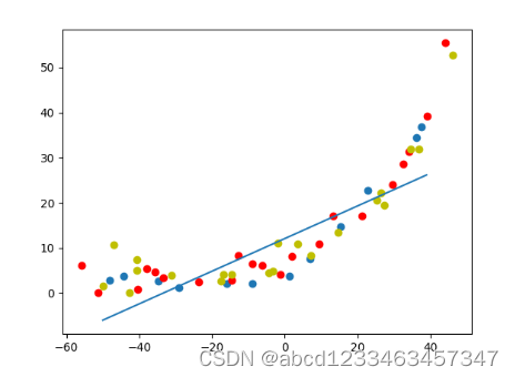
第一步：使用正则化线性回归进行曲线拟合

在这里插入图片描述

import matplotlib.pyplot as plt
import numpy as np
from scipy import io
from scipy import optimize as opt

"""
利用最简单的正则化的线性回归函数学习bias与varience
"""

#1.读取数据
dt = io.loadmat("E:\机器学习\吴恩达\data_sets\ex5data1.mat")

#测试集
x_train = dt["X"] #(12, 1)
y_train = dt["y"] #(12, 1)
m_train = x_train.shape[0] #12
features = x_train.shape[1] #1


#训练集
x_test = dt["Xtest"] #(21, 1)
y_test = dt["ytest"] #(21, 1)

#验证集
x_val = dt["Xval"] #(21, 1)
y_val = dt["yval"] #(21, 1)

#2.数据可视化
plt.scatter(x_train,y_train)
plt.scatter(x_test,y_test,c="r")
plt.scatter(x_val,y_val,c="y")


#3.定义代价函数与梯度函数

#定义正则化的代价函数
def costFunctionRegularzation(theta,x,y,lamda = 1):
    # 注意：这里得到的h是行向量(12,)
    # 而这里的y是列向量(12,1)
    # 如果直接h-y会得到一个（12,12）的矩阵
    h = theta @ x.T  # (12,)
    cost0_temp = 1/(2*m_train)* np.sum(np.power((h - y.T), 2))
    reg_temp = lamda / (2*m_train) * np.sum(np.power(theta[1:],2))
    return cost0_temp+reg_temp

# print(costFunctionRegularzation(theta,x_train,y_train))


#定义正则化的梯度函数
def gradientRegularzation(theta,x,y,lamda = 1):
    h = theta @ x.T #(12,)
    #print(y.flatten().shape) #(12,)
    #注意：这里不能用h-y.T，因为这样最后gradient的类型是(1,2)的二维array，与theta类型不一致
    gradient = 1 / m_train * ((h - y.flatten()) @ x) + lamda / m_train * theta #(2,)
    return gradient


#print(gradientRegularzation(theta, x_train, y_train)) #[[-15.21968234 598.25074417]]

def plot_fit(theta):
    x = np.arange(-50, 40, step=1)
    y = theta[0]+theta[1]*x
    plt.plot(x, y)
    plt.show

#4.调用函数
temp = np.ones((m_train,1))
x_train = np.concatenate((temp,x_train),1)
theta = np.array([1,1]) #(2, )

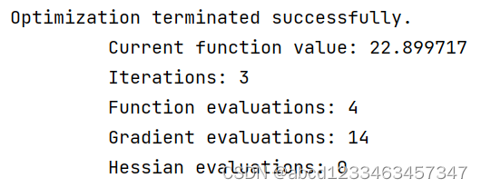
result0 = opt.fmin_ncg(f = costFunctionRegularzation , fprime = gradientRegularzation , x0 = theta , args = (x_train,y_train),maxiter=400)

#展示拟合曲线
plot_fit(result0)
plt.show()

第二步：画出学习曲线，对偏差-方差问题进行诊断。

从没有正则化，且只有两个特征的情况下的学习曲线可以看出，验证误差与训练误差逐渐接近且非常稳定，所以处于高偏差，欠拟合的状态。

在这里插入图片描述

#计算出学习曲线所需的横轴与纵轴
def learning_curve(x,y):
    train_temp = np.zeros(m_train) #(12,)
    val_temp = np.zeros(m_train) #(21,)
    test_temp = np.zeros(m_train) #(21,)
    for i in range(1,m_train+1):
        theta_init =  np.ones(2)
        x_temp = x[0:i,:]
        y_temp = y[0:i]
        theta_temp = opt.fmin_ncg(f = costFunctionRegularzation,fprime=gradientRegularzation,x0 = theta_init,args=(x_temp,y_temp,0),maxiter=400) #(2,)
        train_temp[i-1] = costFunctionRegularzation(theta_temp,x_temp,y_temp)
        val_temp[i-1] = costFunctionRegularzation(theta_temp,x_val,y_val)
        test_temp[i-1] = costFunctionRegularzation(theta_temp, x_test, y_test)
    x_line = np.arange(1,m_train+1)
    plt.plot(x_line,train_temp)
    plt.plot(x_line,val_temp,c = "r")
    plt.plot(x_line,test_temp,c = "y")


x_train = addOne(x_train)
x_val = addOne(x_val)
x_test = addOne(x_test)
learning_curve(x_train,y_train)
plt.show()

第三步：特征映射与标准化

从有正则化且特征数目有7个且标准化的学习曲线中可以看出，验证误差与训练误差之间还是存在不小的差距，所以处于高方差，过拟合的状态下。

注意点：对于验证集与测试集进行标准化时，应该使用测试集的平均值与方差

在这里插入图片描述

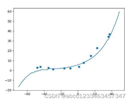
#第三步：特征映射与标准化，要注意：这里的lamda正则化项一定不能为0
#进行特征映射，将x映射成x的n次方组合的矩阵
def mapping(x,n):
    temp = x
    for i in range(2,n+1):
        temp = np.concatenate((temp,np.power(x,i)),1)
    return temp

#标准化
def normalization(x):
    sigma = np.std(x, axis=0, ddof=1)  # axis=0计算每一列的标准差,ddof=1表示自由度为N-1
    ave = np.mean(x, axis=0)
    x = (x - ave) / sigma
    return x, ave, sigma

map_n = 6
xtrain,average_train,std_train = normalization(mapping(x_train,map_n))
xtrain = addOne(xtrain) #(12,7)
theta_mapping = opt.fmin_ncg(f = costFunctionRegularzation,fprime=gradientRegularzation,x0=np.ones(map_n+1),args=(xtrain,y_train,1),maxiter=400)


#绘制出拟合曲线
x_line = np.arange(-70,50,step=1).reshape(120,1)
#注意这里要对x_line标准化
x_temp = (mapping(x_line,map_n)- average_train)/std_train #这里的x要同样进行特征映射和标准化
x_temp = addOne(x_temp) #(120,7)
y_temp = x_temp @ theta_mapping #(120,)

plt.scatter(x_train,y_train)
plt.plot(x_line,y_temp)
plt.show()



#绘制出学习曲线
xval = mapping(x_val,map_n)
xval = (xval-average_train)/std_train
xval = addOne(xval)
xtest = mapping(x_test,map_n)
xtest = (xtest-average_train)/std_train
xtest = addOne(xtest)

learning_curve(xtrain,y_train,xval,y_val,xtest,y_test)
plt.show()

第四步：选择合适的正则化参数

选择10个不同的lamda值，画出训练误差与验证误差关于lamda的函数，可知lamda=1时，验证误差最小。

（我看参考链接里说应该是lamda=3时验证误差最小，因为对验证集标准化时要用训练集的平均值与标准方差，但是我对验证集标准化时使用了训练集的平均值与标准方差，还是和原来博主的结果一样）

在这里插入图片描述

#第四步：选择合适的正则化参数
lamdas = np.array([0,0.001,0.003,0.01,0.03,0.1,0.3,1,3,10])
val_error = np.zeros(10)
train_error = np.zeros(10)
map_n = 6
xtrain,average_train,std_train = normalization(mapping(x_train,map_n))
xtrain = addOne(xtrain) #(12,7)
xval = mapping(x_val,map_n)
xval = (xval-average_train)/std_train
xval = addOne(xval)
xtest = mapping(x_test,map_n)
xtest = (xtest-average_train)/std_train
xtest = addOne(xtest)

for i in range(10):
    theta_lamda = opt.fmin_ncg(f = costFunctionRegularzation,fprime=gradientRegularzation,x0 = np.ones(map_n+1),args=(xtrain,y_train,lamdas[i]),maxiter=400)
    #注意：这里计算代价函数时，应该让正则化参数为0
    val_error[i] = costFunctionRegularzation(theta_lamda,xtrain,y_train,0)
    train_error[i] = costFunctionRegularzation(theta_lamda,xval,y_val,0)

plt.plot(lamdas,train_error,c="r",label = "train")
plt.plot(lamdas,val_error,c="y",label = "val")
plt.show()