


 文章介绍了R语言在生物信息学统计分析中的重要性,包括数据清洗、预处理、数据可视化、数据分析、数据挖掘等方面的应用,并通过实例展示了如何使用R进行单样本均值检验、独立两样本t检验、比例检验、方差的假设检验、拟合优度检验、非参数检验、回归分析等统计方法。
Introduction
统计分析在生物信息学中具有非常重要的意义,因为生物信息学研究的数据量庞大、复杂性高,而统计分析可以帮助我们更好地理解和解释这些数据。下面是统计分析对生物信息学的几个重要意义:
- 数据清洗和预处理:生物信息学研究中经常需要处理大规模的数据,而这些数据可能存在噪声、错误和缺失值等问题。统计分析可以帮助我们对数据进行清洗和预处理,以确保数据的质量和可靠性。
- 数据可视化:统计分析可以帮助我们将复杂的数据转化为可视化图形,从而更好地理解数据的分布、关系和趋势。这些图形可以帮助我们发现隐藏在数据中的模式和规律。
- 数据分析:生物信息学研究中需要对大量的数据进行分析,例如比较基因组学、转录组学、蛋白质组学等。统计分析可以帮助我们对数据进行建模和预测,从而深入探究生物学的复杂现象和机制。
- 数据挖掘:生物信息学研究中需要挖掘大量的数据来发现新的生物学现象和机制。统计分析可以帮助我们从数据中提取出有用的信息和知识,进而推动生物学的研究和发展。
R语言是一个专门用于数据分析和统计建模的编程语言,它有以下几个优点,使其成为做统计分析的理想选择:
-
免费和开源:R语言是一个免费和开源的软件,可以在不付出额外成本的情况下使用和定制。这使得许多学生、学者和数据分析师选择R语言作为他们的首选统计分析工具。
-
强大的数据处理能力:R语言具有强大的数据处理能力,支持多种数据结构和数据类型,可以轻松地进行数据清洗、整合、变换和分析。
-
丰富的统计分析函数库:R语言具有丰富的统计分析函数库,包括线性回归、逻辑回归、聚类分析、主成分分析、时间序列分析等等。这些函数库提供了许多常用的统计分析方法,可以满足不同数据分析需求。
-
图形可视化功能:R语言具有强大的图形可视化功能,可以轻松地创建各种类型的图表,包括散点图、条形图、折线图、热图等。这些图表可以帮助数据分析师更好地理解数据、发现规律和提取信息。
-
社区支持和生态系统:R语言拥有庞大的用户社区和生态系统,用户可以轻松地找到并使用数千种可用的统计分析工具和R包,这些工具和R包可以帮助用户更加高效地完成统计分析任务。
我想在这里稍微记录一下我使用R常用的一些初等统计分析方法,如回归,方差分析,广义线性模型等,主要参考资料是《R语言教程》 VII部分统计分析的内容。
Statistics
基础用法
单样本均值检验
?t.test()
#install.packages("ggstatsplot",dependencies = T)
library(ggstatsplot)
#这个包会在画图的过程中计算很多统计量,帮我们更好地把握数据的性质
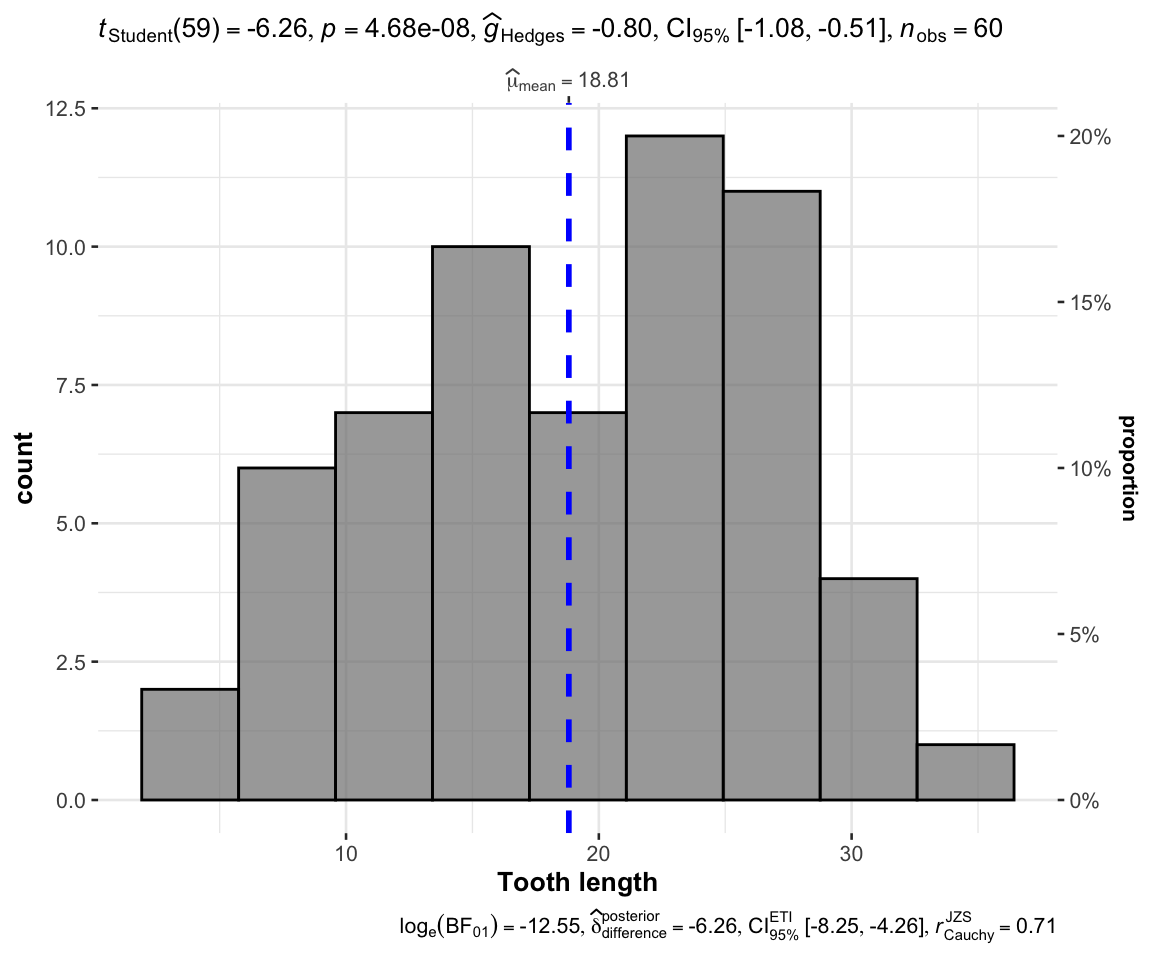
#比如我们想看tooth length均值是否和25有显著差异
t.test(ToothGrowth$len,mu = 25,alternative = "two.sided")
##
## 	One Sample t-test
##
## data:  ToothGrowth$len
## t = -6.2648, df = 59, p-value = 0.00000004681
## alternative hypothesis: true mean is not equal to 25
## 95 percent confidence interval:
##  16.83731 20.78936
## sample estimates:
## mean of x
##  18.81333
gghistostats(
  data            = ToothGrowth,
  x               = len,
  xlab            = "Tooth length",
  test.value = 25
)
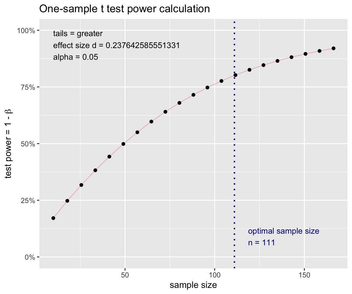
检验的功效, 是指对立假设成立时检验拒绝 H 0 H_0 H0的概率 1 − β 1-\beta 1−β, 其中 β \beta β是第二类错误, 即当对立假设成立时错误地接受 H 0 H_0 H0的概率。 需要足够大的样本量才能使得检验能够发现实际存在的显著差异。
pwr::pwr.t.test(
  type = "one.sample",
  alternative="greater",
  d = (7.25 - 7.0)/1.052,
  sig.level = 0.05,
  power = 0.80 ) |>
  plot()
均值比较
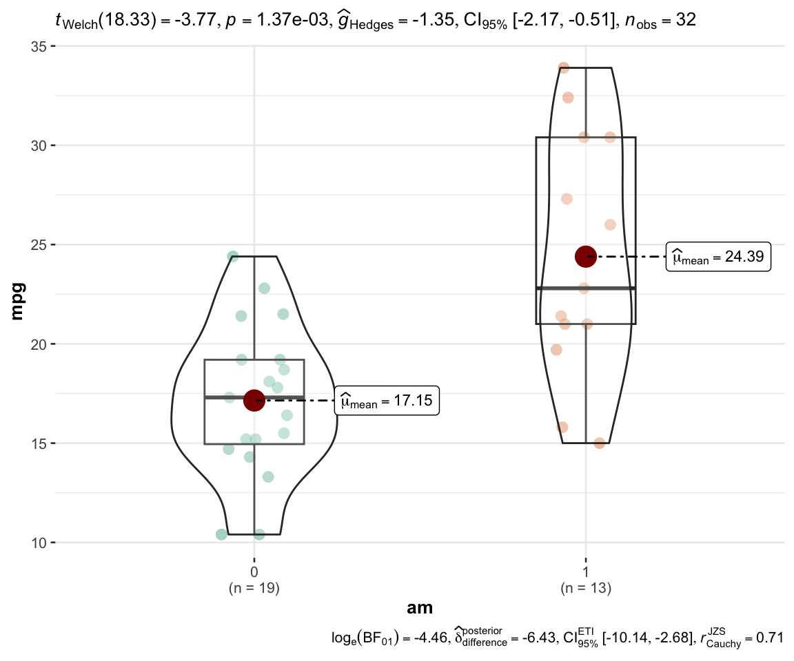
独立两样本t检验
t.test(mpg~am,data = mtcars)
##
## 	Welch Two Sample t-test
##
## data:  mpg by am
## t = -3.7671, df = 18.332, p-value = 0.001374
## alternative hypothesis: true difference in means between group 0 and group 1 is not equal to 0
## 95 percent confidence interval:
##  -11.280194  -3.209684
## sample estimates:
## mean in group 0 mean in group 1
##        17.14737        24.39231
ggbetweenstats(mtcars, am, mpg)
比例检验
#抽查400个样本100个异常,异常比例是否显著大于0.2
prop.test(100, 400, p=0.20, alternative = "greater")
##
## 	1-sample proportions test with continuity correction
##
## data:  100 out of 400, null probability 0.2
## X-squared = 5.9414, df = 1, p-value = 0.007395
## alternative hypothesis: true p is greater than 0.2
## 95 percent confidence interval:
##  0.2149649 1.0000000
## sample estimates:
##    p
## 0.25
#两次抽查的比例是否一致
prop.test(c(35,27), c(250,300), alternative = "two.sided")
##
## 	2-sample test for equality of proportions with continuity correction
##
## data:  c(35, 27) out of c(250, 300)
## X-squared = 2.9268, df = 1, p-value = 0.08712
## alternative hypothesis: two.sided
## 95 percent confidence interval:
##  -0.007506845  0.107506845
## sample estimates:
## prop 1 prop 2
##   0.14   0.09
方差的假设检验
检查两组数据的方差有误显著差异?
var.test(c(
  20.5, 18.8, 19.8, 20.9, 21.5, 19.5, 21.0, 21.2), c(
  17.7, 20.3, 20.0, 18.8, 19.0, 20.1, 20.2, 19.1),
  alternative = "two.sided")
##
## 	F test to compare two variances
##
## data:  c(20.5, 18.8, 19.8, 20.9, 21.5, 19.5, 21, 21.2) and c(17.7, 20.3, 20, 18.8, 19, 20.1, 20.2, 19.1)
## F = 1.069, num df = 7, denom df = 7, p-value = 0.9322
## alternative hypothesis: true ratio of variances is not equal to 1
## 95 percent confidence interval:
##  0.214011 5.339386
## sample estimates:
## ratio of variances
##           1.068966
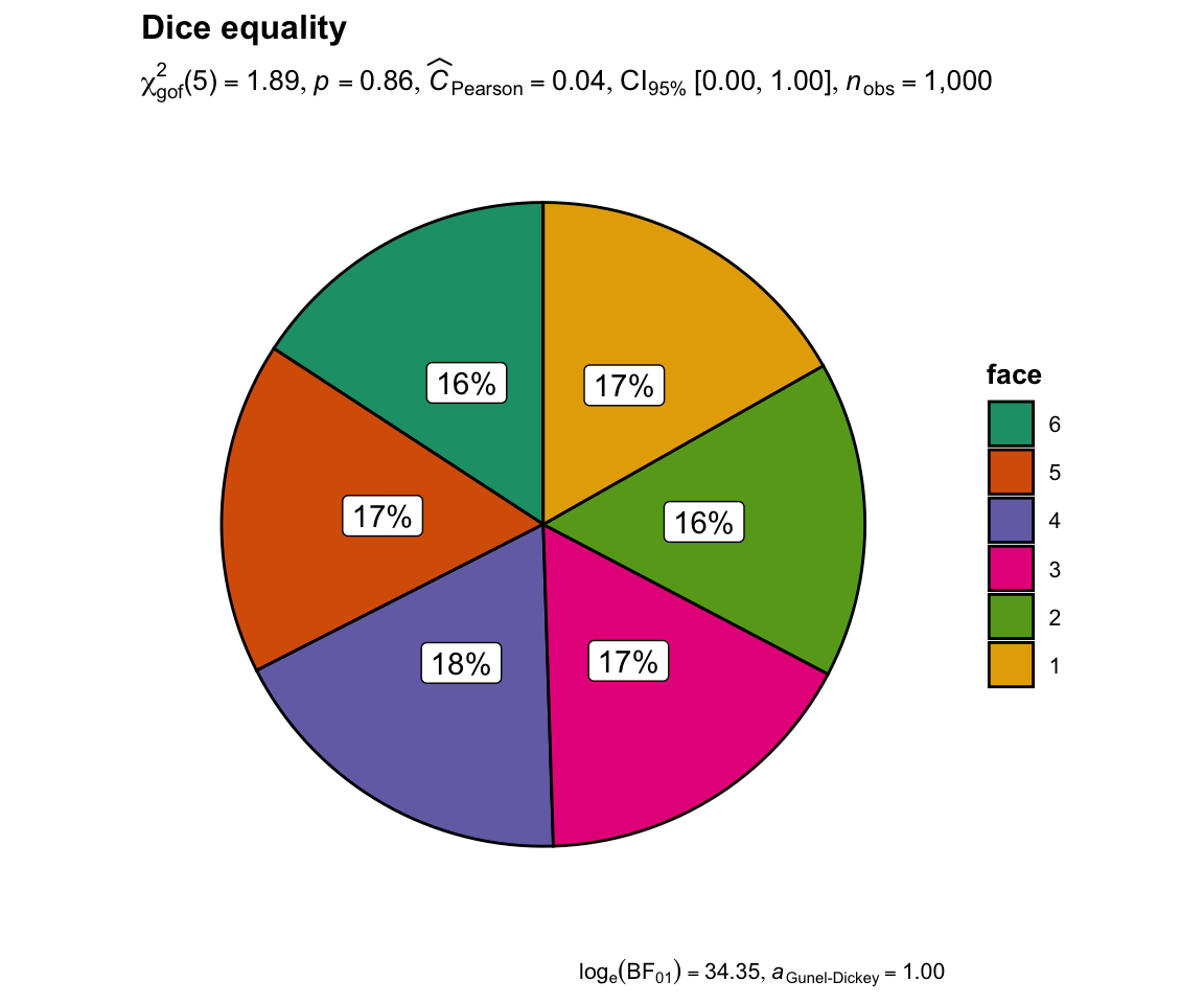
拟合优度检验
#6类face的count比例是否相等,卡方检验
chisq.test(c(168, 159, 168, 180, 167, 158))
##
## 	Chi-squared test for given probabilities
##
## data:  c(168, 159, 168, 180, 167, 158)
## X-squared = 1.892, df = 5, p-value = 0.8639
ggpiestats(
  data         = data.frame(face=1:6,
                 counts=c(168, 159, 168, 180, 167, 158)),
  x            = face,
  counts       = counts,
  title        = "Dice equality"
)
#各类比例是否为指定值
chisq.test(c(48, 98, 54), p=c(0.3, 0.5, 0.2))
##
## 	Chi-squared test for given probabilities
##
## data:  c(48, 98, 54)
## X-squared = 7.34, df = 2, p-value = 0.02548
检验分布类型
vcd包提供了一个goodfit函数, 可以用来拟合指定的某种理论分布(包括泊松、二项、负二项分布), 并检验服从该理论分布的零假设。
set.seed(101)
datax <- rpois(100, 2)
summary(vcd::goodfit(datax, "poisson"))
##
## 	 Goodness-of-fit test for poisson distribution
##
##                       X^2 df  P(> X^2)
## Likelihood Ratio 4.289456  5 0.5085374
独立性卡方检验
ctab.beer <- rbind(c(
  20, 40, 20),
  c(30,30,10))
colnames(ctab.beer) <- c("Light", "Regular", "Dark")
rownames(ctab.beer) <- c("Male", "Female")
addmargins(ctab.beer)
##        Light Regular Dark Sum
## Male      20      40   20  80
## Female    30      30   10  70
## Sum       50      70   30 150
#列联表独立性检验:
chisq.test(ctab.beer)
##
## 	Pearson's Chi-squared test
##
## data:  ctab.beer
## X-squared = 6.1224, df = 2, p-value = 0.04683
#在0.05水平下认为啤酒类型偏好与性别有关
非参数检验
常用的有独立两样本比较的Wilcoxon秩和检验, 单样本的符号秩检验和符号检验等
x <- c(0.80, 0.83, 1.89, 1.04, 1.45, 1.38, 1.91, 1.64, 0.73, 1.46)
y <- c(1.15, 0.88, 0.90, 0.74, 1.21)
wilcox.test(x,mu = 0.7)
##
## 	Wilcoxon signed rank exact test
##
## data:  x
## V = 55, p-value = 0.001953
## alternative hypothesis: true location is not equal to 0.7
wilcox.test(x, y, alternative = "g")
##
## 	Wilcoxon rank sum exact test
##
## data:  x and y
## W = 35, p-value = 0.1272
## alternative hypothesis: true location shift is greater than 0
回归分析
相关分析
- Pearson相关系数:
ρ ( X , Y ) = E [ ( X − E ( X ) ) ( Y − E ( Y ) ) ] V a r ( X ) V a r ( Y ) \rho(X,Y)=\frac{E[(X-E(X))(Y-E(Y))]}{\sqrt{Var(X)Var(Y)}} ρ(X,Y)=Var(X)Var(Y)E[(X−E(X))(Y−E(Y))]
相关系数绝对值在0.8以上认为高度相关。
在0.5到0.8之间认为中度相关。
在0.3到0.5之间认为低度相关。
在0.3以下认为不相关或相关性很弱以至于没有实际价值。
当然,在特别重要的问题中, 只要经过检验显著不等于零的相关都认为是有意义的。
相关系数检验:
检验统计量:
t
=
r
n
−
2
1
−
r
2
t=\frac{r\sqrt{n-2}}{\sqrt{1-r^2}}
t=1−r2rn−2
p值为:
P
(
∣
t
(
n
−
2
)
∣
>
∣
t
0
∣
)
P(|t(n-2)|>|t_0|)
P(∣t(n−2)∣>∣t0∣)
set.seed(1)
x <- runif(30, 0, 10)
xx <- seq(0, 10, length.out = 100)
y <- 40 - (x-7)^2 + rnorm(30)
yy <- 40 - (xx-7)^2
plot(x, y, pch=16)
lines(xx, yy)
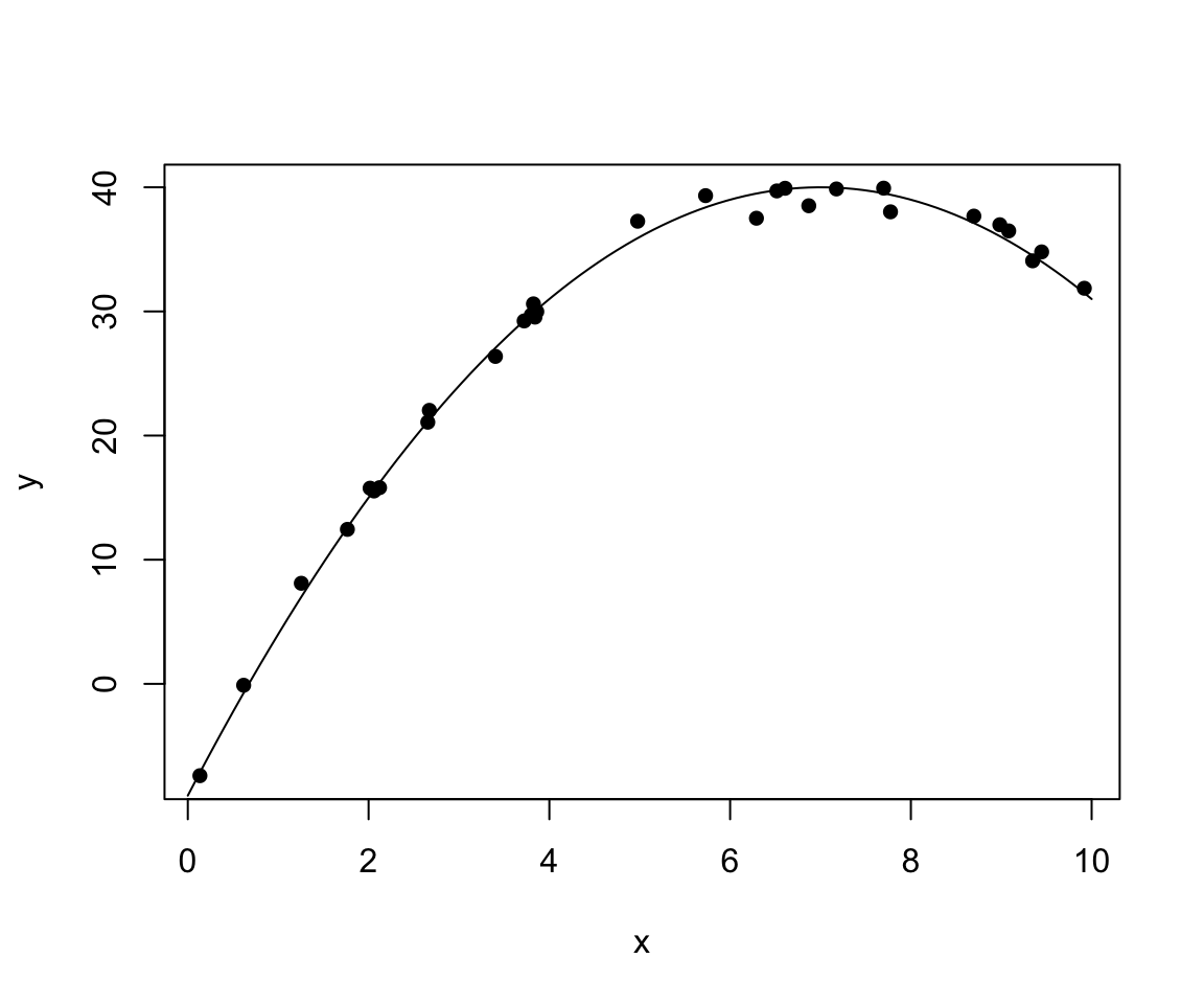
cor(x,y,method = "pearson")
## [1] 0.8244374
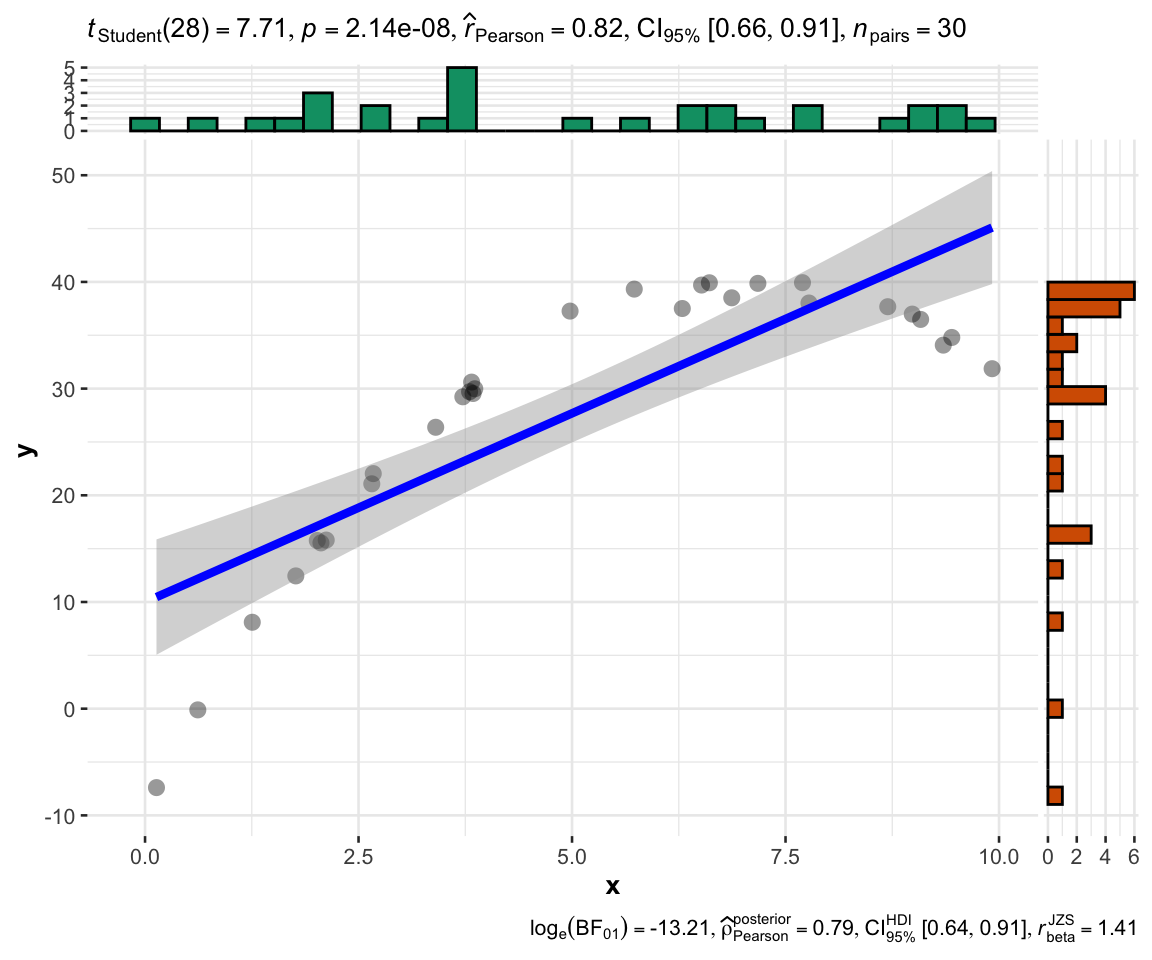
cor.test(x,y,method = "pearson")
##
## 	Pearson's product-moment correlation
##
## data:  x and y
## t = 7.7083, df = 28, p-value = 0.00000002136
## alternative hypothesis: true correlation is not equal to 0
## 95 percent confidence interval:
##  0.6602859 0.9134070
## sample estimates:
##       cor
## 0.8244374
ggstatsplot::ggscatterstats(
    data = data.frame(x,y),
  x     = x,
  y     = y
)
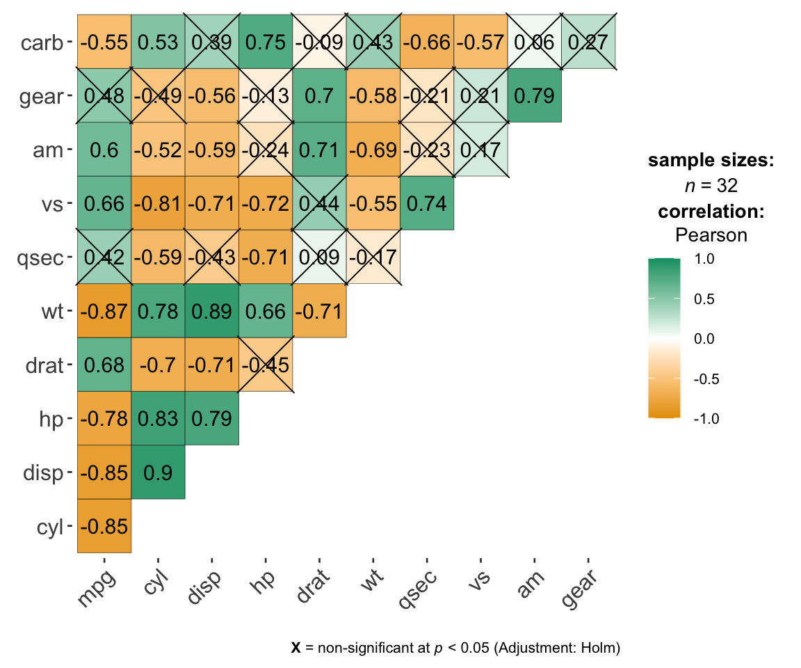
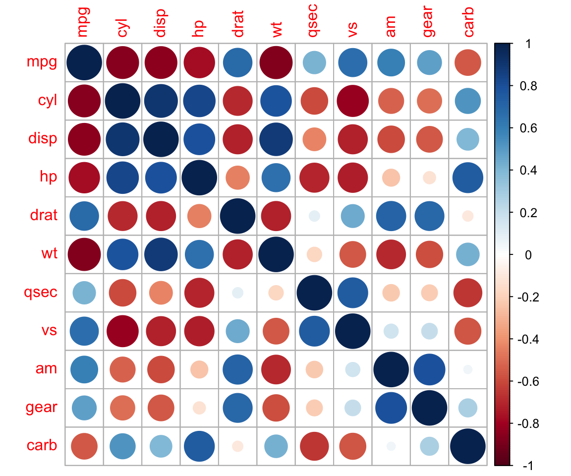
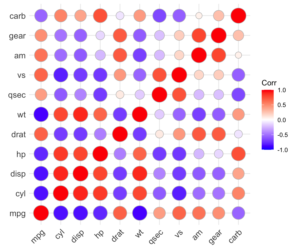
 相关性矩阵,`n*n`或`n*m`的$r$ 和$p-value$矩阵
ggstatsplot::ggcorrmat(
  data     = mtcars
)
pcutils::cor_plot(mtcars)
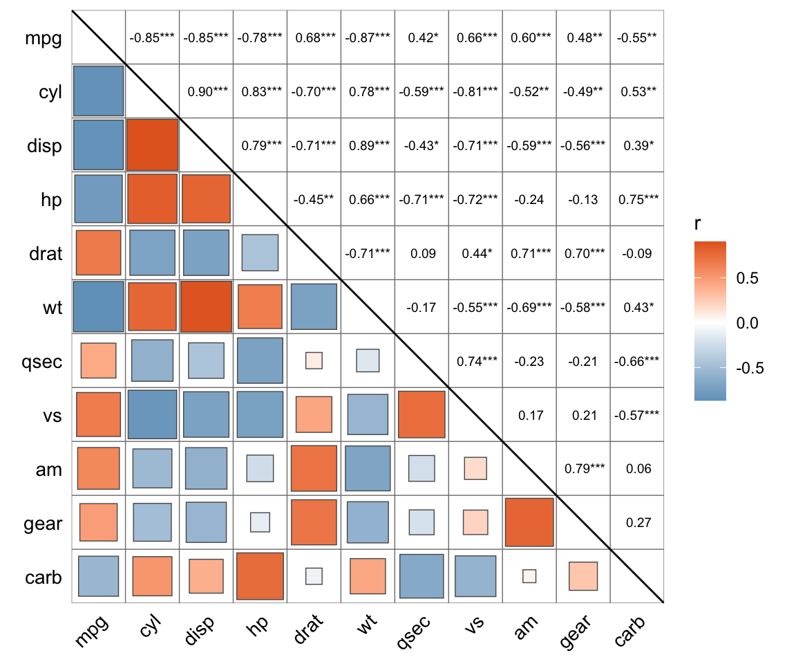
corrplot::corrplot(cor(mtcars))
ggcorrplot::ggcorrplot(cor(mtcars),method = "circle")
-
Spearman秩相关系数
Spearman rho系数, 是两个变量的秩统计量的相关系数 -
Kendall tau系数
当变量正相关性很强时, 任意两个观测的X值的大小顺序应该与Y值的大小顺序相同; 如果独立, 一对观测的X值比较和Y值比较顺序相同与顺序相反的数目应该基本相同。Kandall tau系数也是取值于区间[-1,1], 用这样的思想表示两个变量的相关性和正负。
cor.test(x,y,method = "spearman")
##
## 	Spearman's rank correlation rho
##
## data:  x and y
## S = 922, p-value = 0.000001339
## alternative hypothesis: true rho is not equal to 0
## sample estimates:
##       rho
## 0.7948832
cor.test(x,y,method = "kendall")
##
## 	Kendall's rank correlation tau
##
## data:  x and y
## T = 354, p-value = 0.000000159
## alternative hypothesis: true tau is not equal to 0
## sample estimates:
##       tau
## 0.6275862
一元回归
Y = a + b X + ε , ε ∼ N ( 0 , σ 2 ) Y=a+bX+\varepsilon, \varepsilon \sim N(0,\sigma^2) Y=a+bX+ε,ε∼N(0,σ2)
最小二乘法
b
^
=
∑
i
(
x
i
−
x
‾
)
(
y
i
−
y
‾
)
∑
i
(
x
−
x
i
)
2
=
r
x
y
S
y
S
x
\hat{b}=\frac{\sum_i(x_i-\overline{x})(y_i-\overline{y})}{\sum_i{(x-x_i)}^2}=r_{xy}\frac{S_y}{S_x}
b^=∑i(x−xi)2∑i(xi−x)(yi−y)=rxySxSy
a
^
=
y
‾
−
b
^
x
‾
\hat{a}=\overline{y}-\hat{b}\overline{x}
a^=y−b^x
回归有效性可以用
R
2
R^2
R2和
p
−
v
a
l
u
i
e
p-valuie
p−valuie来度量,
R
2
=
1
−
S
S
E
S
S
T
R^2=1-\frac{SSE}{SST}
R2=1−SSTSSE
统计量 F = S S R S S E / ( n − 2 ) F=\frac{SSR}{SSE/(n-2)} F=SSE/(n−2)SSR, p − v a l u e p-value p−value为 P ( F ( 1 , n − 2 ) > c ) P(F(1,n-2)>c) P(F(1,n−2)>c),c为F的值。
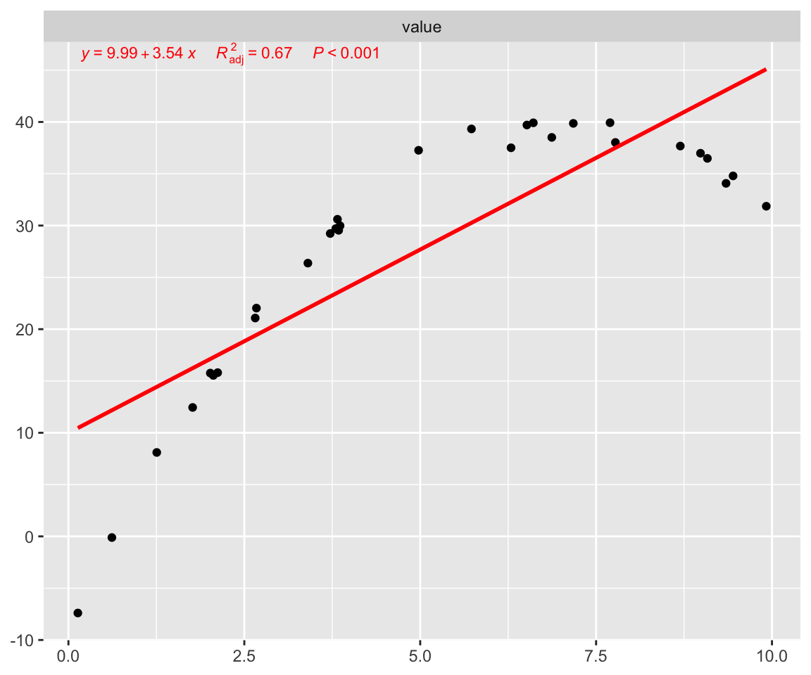
lm1 <- lm(y ~ x)
summary(lm1)
##
## Call:
## lm(formula = y ~ x)
##
## Residuals:
##     Min      1Q  Median      3Q     Max
## -17.856  -4.549   2.141   6.048   9.664
##
## Coefficients:
##             Estimate Std. Error t value     Pr(>|t|)
## (Intercept)   9.9855     2.6930   3.708     0.000914 ***
## x             3.5396     0.4592   7.708 0.0000000214 ***
## ---
## Signif. codes:  0 '***' 0.001 '**' 0.01 '*' 0.05 '.' 0.1 ' ' 1
##
## Residual standard error: 7.302 on 28 degrees of freedom
## Multiple R-squared:  0.6797,	Adjusted R-squared:  0.6683
## F-statistic: 59.42 on 1 and 28 DF,  p-value: 0.00000002136
#prediction
predict(lm1,newdata =data.frame(x=c(5,10,15)))
##        1        2        3
## 27.68364 45.38182 63.08000
pcutils::my_lm(y,x)
多元回归
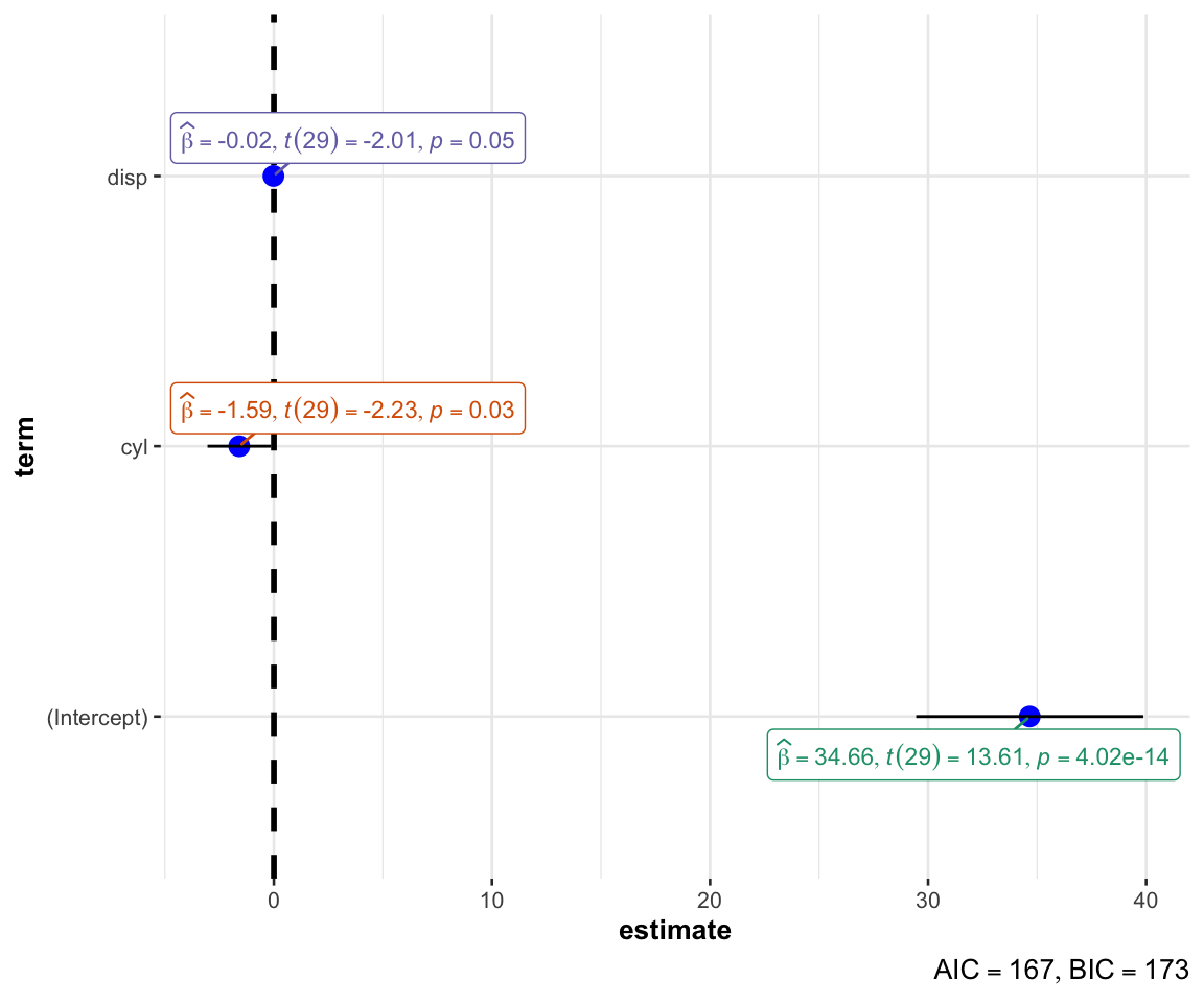
lm2 <- lm(mpg ~ cyl + disp, data=mtcars)
summary(lm2)
##
## Call:
## lm(formula = mpg ~ cyl + disp, data = mtcars)
##
## Residuals:
##     Min      1Q  Median      3Q     Max
## -4.4213 -2.1722 -0.6362  1.1899  7.0516
##
## Coefficients:
##             Estimate Std. Error t value Pr(>|t|)
## (Intercept) 34.66099    2.54700  13.609 4.02e-14 ***
## cyl         -1.58728    0.71184  -2.230   0.0337 *
## disp        -0.02058    0.01026  -2.007   0.0542 .
## ---
## Signif. codes:  0 '***' 0.001 '**' 0.01 '*' 0.05 '.' 0.1 ' ' 1
##
## Residual standard error: 3.055 on 29 degrees of freedom
## Multiple R-squared:  0.7596,	Adjusted R-squared:  0.743
## F-statistic: 45.81 on 2 and 29 DF,  p-value: 0.000000001058
ggstatsplot::ggcoefstats(lm2)
#回归自变量筛选
lm3 <- step(lm(mpg ~ cyl + disp+hp+drat+vs, data=mtcars))
## Start:  AIC=77.08
## mpg ~ cyl + disp + hp + drat + vs
##
##        Df Sum of Sq    RSS    AIC
## - vs    1    0.3134 244.90 75.124
## - cyl   1    7.6839 252.27 76.073
## - drat  1   14.3330 258.92 76.905
## - disp  1   14.6709 259.26 76.947
## <none>              244.59 77.083
## - hp    1   19.8255 264.41 77.577
##
## Step:  AIC=75.12
## mpg ~ cyl + disp + hp + drat
##
##        Df Sum of Sq    RSS    AIC
## - cyl   1     8.444 253.35 74.209
## - disp  1    14.765 259.67 74.997
## <none>              244.90 75.124
## - drat  1    16.467 261.37 75.206
## - hp    1    19.613 264.51 75.589
##
## Step:  AIC=74.21
## mpg ~ disp + hp + drat
##
##        Df Sum of Sq    RSS    AIC
## <none>              253.35 74.209
## - drat  1    30.148 283.49 75.806
## - disp  1    38.107 291.45 76.693
## - hp    1    49.550 302.90 77.925
多重共线性
狭义的多重共线性(multicollinearity): 自变量的数据存在线性组合近似地等于零, 使得解线性方程组求解回归系数时结果不稳定, 回归结果很差。
广义的多重共线性: 自变量之间存在较强的相关性, 这样自变量是联动的, 互相之间有替代作用。 甚至于斜率项的正负号都因为这种替代作用而可能是错误的方向。
#car包的vif()函数计算方差膨胀因子
car::vif(lm3)
##     disp       hp     drat
## 4.621988 2.868264 2.166843
非参数回归
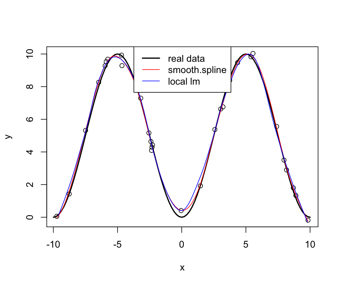
所谓参数回归, 是指回归函数有预先确定的公式, 仅需要估计的未知参数; 非参数回归, 就是没有预先确定的公式, 的形式本身也依赖于输入的样本, 。 下面描述的核回归就是这样典型的非参数回归, 样条平滑、样条函数回归一般也看作是非参数回归。
#样条平滑
set.seed(1)
nsamp <- 30
x <- runif(nsamp, -10, 10)
xx <- seq(-10, 10, length.out=100)
x <- sort(x)
y <- 10*sin(x/10*pi)^2 + rnorm(nsamp,0,0.3)
plot(x, y)
curve(10*sin(x/10*pi)^2, -10, 10, add=TRUE, lwd=2)

library(splines)
res <- smooth.spline(x, y)
lines(spline(res$x, res$y), col="red")
res2 <- loess(y ~ x, degree=2, span=0.3)
lines(xx, predict(res2, newdata=data.frame(x=xx)),
      col="blue")
legend("top", lwd=c(2,1,1),
       col=c("black", "red", "blue"),
       legend=c("real data", "smooth.spline", "local lm"))
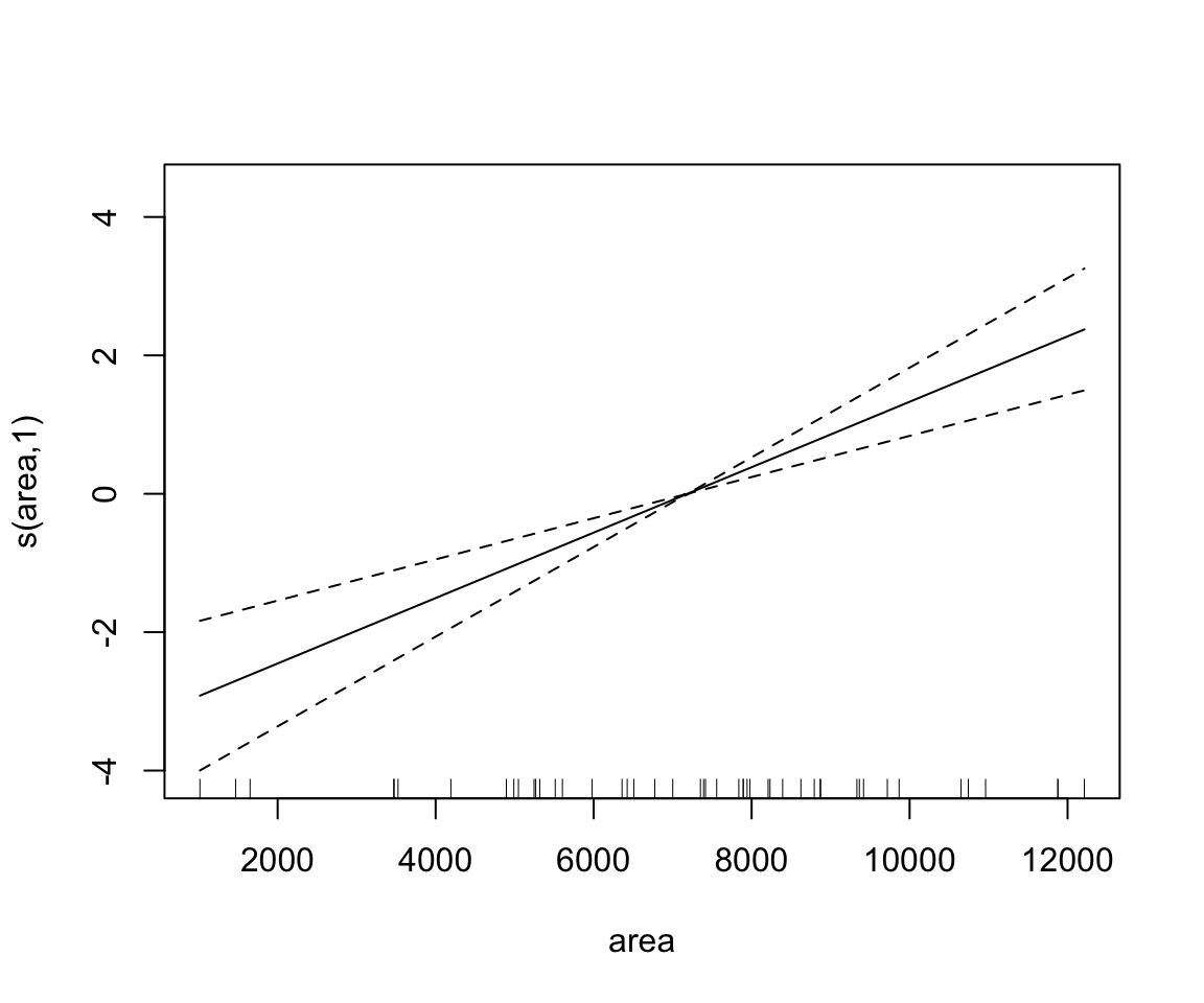
## 线性可加模型
## R扩展包mgcv的gam()函数可以执行这样的可加模型的非参数回归拟合。
lm.rock <- lm(log(perm) ~ area + peri + shape, data=rock)
summary(lm.rock)
##
## Call:
## lm(formula = log(perm) ~ area + peri + shape, data = rock)
##
## Residuals:
##     Min      1Q  Median      3Q     Max
## -1.8092 -0.5413  0.1734  0.6493  1.4788
##
## Coefficients:
##                Estimate  Std. Error t value Pr(>|t|)
## (Intercept)  5.33314499  0.54867792   9.720 1.59e-12 ***
## area         0.00048498  0.00008657   5.602 1.29e-06 ***
## peri        -0.00152661  0.00017704  -8.623 5.24e-11 ***
## shape        1.75652601  1.75592362   1.000    0.323
## ---
## Signif. codes:  0 '***' 0.001 '**' 0.01 '*' 0.05 '.' 0.1 ' ' 1
##
## Residual standard error: 0.8521 on 44 degrees of freedom
## Multiple R-squared:  0.7483,	Adjusted R-squared:  0.7311
## F-statistic:  43.6 on 3 and 44 DF,  p-value: 3.094e-13
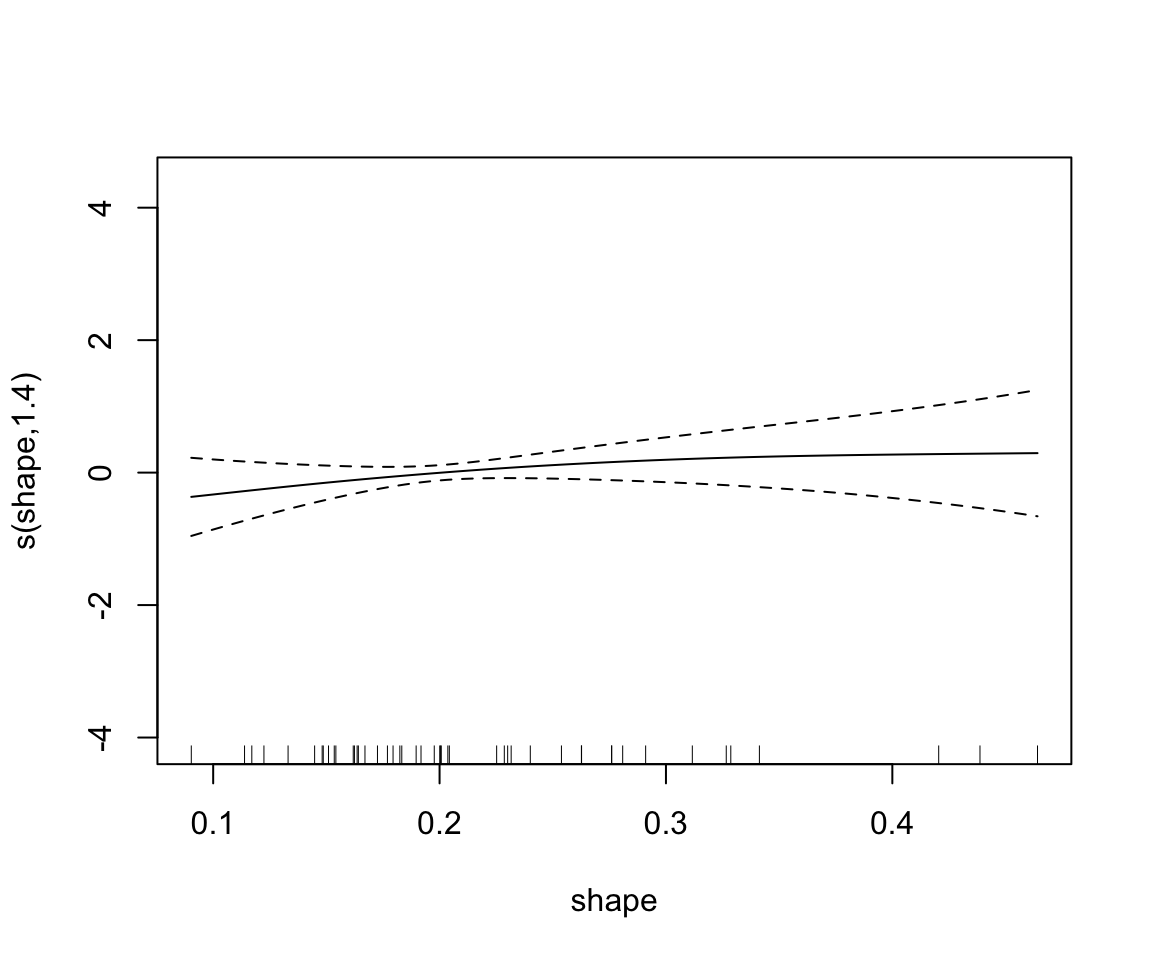
gam.rock1 <- mgcv::gam(log(perm) ~ s(area) + s(peri) + s(shape), data=rock)
summary(gam.rock1)
##
## Family: gaussian
## Link function: identity
##
## Formula:
## log(perm) ~ s(area) + s(peri) + s(shape)
##
## Parametric coefficients:
##             Estimate Std. Error t value Pr(>|t|)
## (Intercept)   5.1075     0.1222   41.81   <2e-16 ***
## ---
## Signif. codes:  0 '***' 0.001 '**' 0.01 '*' 0.05 '.' 0.1 ' ' 1
##
## Approximate significance of smooth terms:
##            edf Ref.df     F    p-value
## s(area)  1.000  1.000 29.13 0.00000307 ***
## s(peri)  1.000  1.000 71.30    < 2e-16 ***
## s(shape) 1.402  1.705  0.58      0.437
## ---
## Signif. codes:  0 '***' 0.001 '**' 0.01 '*' 0.05 '.' 0.1 ' ' 1
##
## R-sq.(adj) =  0.735   Deviance explained = 75.4%
## GCV = 0.78865  Scale est. = 0.71631   n = 48
plot(gam.rock1)

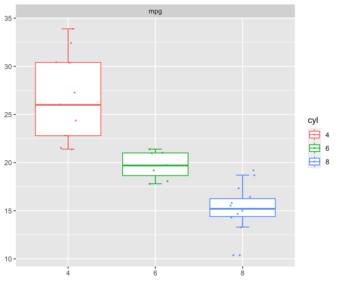
方差分析
单因素方差分析可以看成基础统计中两样本t检验的一个推广, 要比较试验观测值的某个因变量(称为“指标”)按照一个分组变量(称为“因素”)分组后, 各组的因变量均值有无显著差异。
mtcars$cyl=as.factor(mtcars$cyl)
aov.manu <- aov(mpg ~ cyl, data=mtcars)
summary(aov.manu)
##             Df Sum Sq Mean Sq F value        Pr(>F)
## cyl          2  824.8   412.4    39.7 0.00000000498 ***
## Residuals   29  301.3    10.4
## ---
## Signif. codes:  0 '***' 0.001 '**' 0.01 '*' 0.05 '.' 0.1 ' ' 1
pcutils::group_box(mtcars["mpg"],group = "cyl",metadata = mtcars)
#非参数形式
kruskal.test(mpg ~ cyl, data=mtcars)
##
## 	Kruskal-Wallis rank sum test
##
## data:  mpg by cyl
## Kruskal-Wallis chi-squared = 25.746, df = 2, p-value = 0.000002566
进行多个假设检验(如均值比较)的操作称为*“多重比较”*(multiple comparison, 或multiple testing), 多次检验会使得总第一类错误概率增大。
pcutils::multitest(mtcars$mpg,mtcars$cyl)
## ====================================1.ANOVA:====================================
##             Df Sum Sq Mean Sq F value        Pr(>F)
## group        2  824.8   412.4    39.7 0.00000000498 ***
## Residuals   29  301.3    10.4
## ---
## Signif. codes:  0 '***' 0.001 '**' 0.01 '*' 0.05 '.' 0.1 ' ' 1
## ================================2.Kruskal.test:================================
##
## 	Kruskal-Wallis rank sum test
##
## data:  var by group
## Kruskal-Wallis chi-squared = 25.746, df = 2, p-value = 0.000002566
##
## ==========================3.LSDtest, bonferroni p-adj:==========================
##        var groups
## 4 26.66364      a
## 6 19.74286      b
## 8 15.10000      c
## ==================================4.tukeyHSD:==================================
##   Tukey multiple comparisons of means
##     95% family-wise confidence level
##
## Fit: aov(formula = var ~ group)
##
## $group
##           diff        lwr        upr     p adj
## 6-4  -6.920779 -10.769350 -3.0722086 0.0003424
## 8-4 -11.563636 -14.770779 -8.3564942 0.0000000
## 8-6  -4.642857  -8.327583 -0.9581313 0.0112287
##
## =================================5.Wilcox-test:=================================
##               4            6             8
## 4 1.00000000000 0.0006658148 0.00002774715
## 6 0.00066581478 1.0000000000 0.00101304469
## 8 0.00002774715 0.0010130447 1.00000000000
广义线性模型
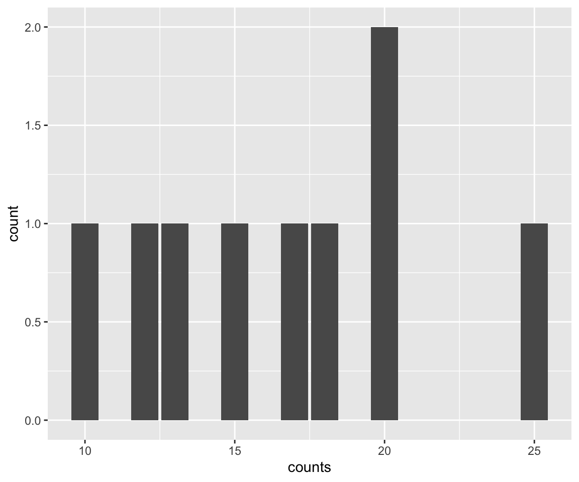
泊松回归
counts <- c(18,17,15,20,10,20,25,13,12)
outcome <- gl(3,1,9)
treatment <- gl(3,3)
D93=data.frame(treatment, outcome, counts) ## showing data

ggplot(data = D93, mapping = aes(x = counts)) +geom_bar()
glm.D93 <- glm(counts ~ outcome + treatment,data = D93, family = poisson())
summary(glm.D93)
##
## Call:
## glm(formula = counts ~ outcome + treatment, family = poisson(),
##     data = D93)
##
## Deviance Residuals:
##        1         2         3         4         5         6         7         8
## -0.67125   0.96272  -0.16965  -0.21999  -0.95552   1.04939   0.84715  -0.09167
##        9
## -0.96656
##
## Coefficients:
##               Estimate Std. Error z value Pr(>|z|)
## (Intercept)  3.045e+00  1.709e-01  17.815   <2e-16 ***
## outcome2    -4.543e-01  2.022e-01  -2.247   0.0246 *
## outcome3    -2.930e-01  1.927e-01  -1.520   0.1285
## treatment2  -3.242e-16  2.000e-01   0.000   1.0000
## treatment3  -2.148e-16  2.000e-01   0.000   1.0000
## ---
## Signif. codes:  0 '***' 0.001 '**' 0.01 '*' 0.05 '.' 0.1 ' ' 1
##
## (Dispersion parameter for poisson family taken to be 1)
##
##     Null deviance: 10.5814  on 8  degrees of freedom
## Residual deviance:  5.1291  on 4  degrees of freedom
## AIC: 56.761
##
## Number of Fisher Scoring iterations: 4
逻辑斯谛回归
….


 被折叠的 条评论
为什么被折叠?
被折叠的 条评论
为什么被折叠?
 到【灌水乐园】发言


