caret教程09：决策树小例子

前面已经铺垫了超多caret的基础知识，所以下面就是具体的实战演示了。

今天给大家演示下caret做决策树的例子，但其实并不是很好用，还不如之前介绍的直接使用rpart，或者tidymodels，mlr3。

加载数据和R包

library(caret)

library(modeldata)
str(penguins)

## tibble [344 × 7] (S3: tbl_df/tbl/data.frame)
##  $ species          : Factor w/ 3 levels "Adelie","Chinstrap",..: 1 1 1 1 1 1 1 1 1 1 ...
##  $ island           : Factor w/ 3 levels "Biscoe","Dream",..: 3 3 3 3 3 3 3 3 3 3 ...
##  $ bill_length_mm   : num [1:344] 39.1 39.5 40.3 NA 36.7 39.3 38.9 39.2 34.1 42 ...
##  $ bill_depth_mm    : num [1:344] 18.7 17.4 18 NA 19.3 20.6 17.8 19.6 18.1 20.2 ...
##  $ flipper_length_mm: int [1:344] 181 186 195 NA 193 190 181 195 193 190 ...
##  $ body_mass_g      : int [1:344] 3750 3800 3250 NA 3450 3650 3625 4675 3475 4250 ...
##  $ sex              : Factor w/ 2 levels "female","male": 2 1 1 NA 1 2 1 2 NA NA ...

用这个企鹅数据集做演示。一共有377行，7列，其中species是结果变量，三分类，因子型，其余列是预测变量。

首先还是简单探索下数据：

library(GGally)

ggbivariate(penguins, "species")

## Warning: Removed 2 rows containing non-finite values (`stat_boxplot()`).
## Removed 2 rows containing non-finite values (`stat_boxplot()`).
## Removed 2 rows containing non-finite values (`stat_boxplot()`).
## Removed 2 rows containing non-finite values (`stat_boxplot()`).

## Warning: Removed 11 rows containing non-finite values (`stat_prop()`).

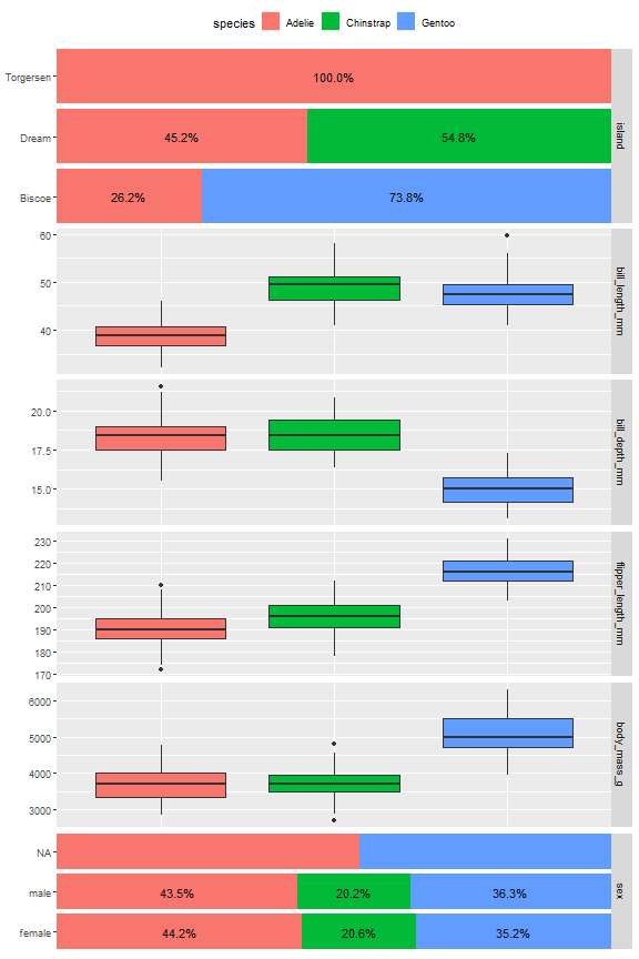
这个数据还可以，sex有一些缺失值，其他看着还行。

预处理

做个简单的预处理，连续性变量中心化，分类变量设置哑变量。预处理这部分不如tidymodels好用。

cent <- preProcess(penguins, method = c("center","scale"))
pen_df <- predict(cent, newdata = penguins)

class <- pen_df$species
dummy <- dummyVars(species ~. , data=pen_df)
pen_df <- predict(dummy, newdata = pen_df)

pen_df <- as.data.frame(pen_df)
pen_df$species <- class

str(pen_df)

## 'data.frame':	344 obs. of  10 variables:
##  $ island.Biscoe    : num  0 0 0 0 0 0 0 0 0 0 ...
##  $ island.Dream     : num  0 0 0 0 0 0 0 0 0 0 ...
##  $ island.Torgersen : num  1 1 1 1 1 1 1 1 1 1 ...
##  $ bill_length_mm   : num  -0.883 -0.81 -0.663 NA -1.323 ...
##  $ bill_depth_mm    : num  0.784 0.126 0.43 NA 1.088 ...
##  $ flipper_length_mm: num  -1.416 -1.061 -0.421 NA -0.563 ...
##  $ body_mass_g      : num  -0.563 -0.501 -1.187 NA -0.937 ...
##  $ sex.female       : num  0 1 1 NA 1 0 1 0 NA NA ...
##  $ sex.male         : num  1 0 0 NA 0 1 0 1 NA NA ...
##  $ species          : Factor w/ 3 levels "Adelie","Chinstrap",..: 1 1 1 1 1 1 1 1 1 1 ...

建立模型

caret是可以调用rpart包实现决策树的，但是只支持一个超参数cp，感觉不如之前介绍的好用：

• 以决策树为例演示超参数调优的基本方法(上)
• 以决策树为例演示超参数调优的基本方法(下)

# 设定种子数
set.seed(3456)

# 根据结果变量的类别多少划分
trainIndex <- createDataPartition(pen_df$species, p = 0.7, 
                                  list = FALSE)
head(trainIndex)

##      Resample1
## [1,]         2
## [2,]         7
## [3,]         8
## [4,]         9
## [5,]        10
## [6,]        12

penTrain <- pen_df[ trainIndex,]
penTest  <- pen_df[-trainIndex,]

dim(penTrain)

## [1] 242  10

dim(penTest)

## [1] 102  10

# 选择重抽样方法，10折交叉验证
trControl <- trainControl(method = "cv", number = 10,
                          classProbs = T
                          )

set.seed(8)
tree_fit <- train(x = pen_df[,-1],
               y = pen_df$species,
               method = "rpart",
               trControl = trControl,
               tuneLength = 20
               )

tree_fit

## CART 
## 
## 344 samples
##   9 predictor
##   3 classes: 'Adelie', 'Chinstrap', 'Gentoo' 
## 
## No pre-processing
## Resampling: Cross-Validated (10 fold) 
## Summary of sample sizes: 310, 309, 310, 309, 310, 310, ... 
## Resampling results across tuning parameters:
## 
##   cp          Accuracy   Kappa    
##   0.00000000  1.0000000  1.0000000
##   0.03399123  1.0000000  1.0000000
##   0.06798246  1.0000000  1.0000000
##   0.10197368  1.0000000  1.0000000
##   0.13596491  1.0000000  1.0000000
##   0.16995614  1.0000000  1.0000000
##   0.20394737  1.0000000  1.0000000
##   0.23793860  1.0000000  1.0000000
##   0.27192982  1.0000000  1.0000000
##   0.30592105  1.0000000  1.0000000
##   0.33991228  1.0000000  1.0000000
##   0.37390351  0.8023203  0.6725971
##   0.40789474  0.8023203  0.6725971
##   0.44188596  0.8023203  0.6725971
##   0.47587719  0.8023203  0.6725971
##   0.50986842  0.8023203  0.6725971
##   0.54385965  0.8023203  0.6725971
##   0.57785088  0.8023203  0.6725971
##   0.61184211  0.8023203  0.6725971
##   0.64583333  0.6525957  0.3976620
## 
## Accuracy was used to select the optimal model using the largest value.
## The final value used for the model was cp = 0.3399123.

plot(tree_fit)

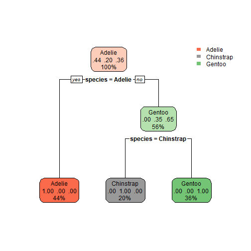
library(rpart.plot)

## Loading required package: rpart

rpart.plot(tree_fit$finalModel)

library(treeheatr)

heat_tree(partykit::as.party(tree_fit$finalModel))

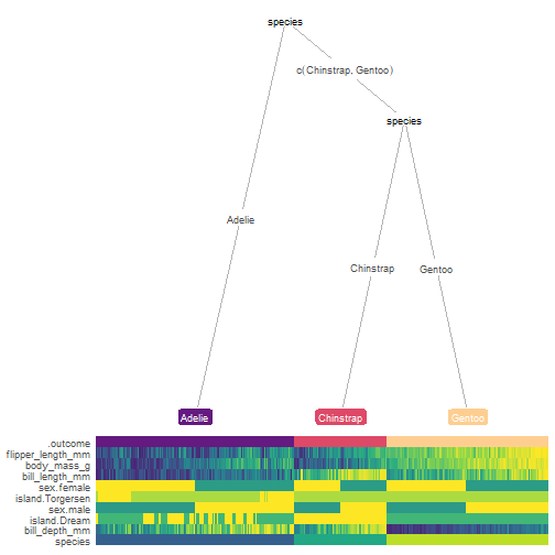
其他图形就不演示了，大家可以参考我们之前的推文。