


获取更多R语言和生信知识,请关注公众号:医学和生信笔记。
公众号后台回复R语言,即可获得海量学习资料!
目录
本系列是对ComplexeHeatmap包的学习笔记,部分内容根据自己的理解有适当的改动,但总体不影响原文。如有不明之处,以原文为准。原文请见:ComplexHeatmap Complete Reference
第一章 简介
复杂热图可用于展示同一个数据集或不同数据集之间的关系或揭示内部规律。ComplexHeatmap包可提供灵活的热图展示及高度自定义的注释图形。
1.1 设计理念
一个完整的热图由热图主体和热图组件构成。热图主体可以被分为不同的行和列,热图组件包括行/列标题,聚类树,行名/列名,行注释条/列注释条。
热图列表由多个热图主体和热图注释组成,但不同的热图主体和注释被有序排列,使得彼此之间具有较好的可比性。
ComplexHeatmap包是面向对象的,主要包括以下类:
-
Heatmap class: 单个热图,包括热图主体,行名/列名,标题,聚类树,行注释条/列注释条;
-
HeatmapList class: 多个热图主体和热图注释;
-
HeatmapAnnotation class: 定义一系列的行注释/列注释,这些注释既可以作为热图组件,又可以独立于热图;
还有一些其他类:
-
SingleAnnotation class: 定义单个行注释/列注释,包含在 HeatmapAnnotation class中;
-
ColorMapping class: 映射颜色,包括热图主体颜色和各种注释的颜色
-
AnnotationFunction class: 创建用户自定义的注释 ComplexHeatmap是基于grid的,充分利用此包需要用户了解grid绘图系统的知识。
1.2 各章节速览
2. 单个热图
介绍单个热图的组成
3. 热图注释
热图注释概念,如何绘制简单注释和复杂注释,简单注释和复杂注释的不同
4. 热图列表
如何绘制多个热图和注释,它们的位置排布是怎样安排的
5. 图例
如何绘制热图主体和注释条的图例,如何自定义图例
6. 热图装饰
如何添加用户自定义图形
7. 瀑布图
8. UpSet plot
9. 其他高阶图形
10. 和其他R包交互
11. 交互式热图
12. 更多例子
第二章 单个热图
单个热图是最常见的可视化图形,虽然ComplexHeatmap包的闪光点是可以同时绘制多个热图,但是作为基本图形,对单个热图的绘制也是很重要的。
首先随机生成一个矩阵
set.seed(123)
nr1 = 4; nr2 = 8; nr3 = 6; nr = nr1 + nr2 + nr3
nc1 = 6; nc2 = 8; nc3 = 10; nc = nc1 + nc2 + nc3
mat = cbind(rbind(matrix(rnorm(nr1*nc1, mean = 1,   sd = 0.5), nr = nr1),
          matrix(rnorm(nr2*nc1, mean = 0,   sd = 0.5), nr = nr2),
          matrix(rnorm(nr3*nc1, mean = 0,   sd = 0.5), nr = nr3)),
    rbind(matrix(rnorm(nr1*nc2, mean = 0,   sd = 0.5), nr = nr1),
          matrix(rnorm(nr2*nc2, mean = 1,   sd = 0.5), nr = nr2),
          matrix(rnorm(nr3*nc2, mean = 0,   sd = 0.5), nr = nr3)),
    rbind(matrix(rnorm(nr1*nc3, mean = 0.5, sd = 0.5), nr = nr1),
          matrix(rnorm(nr2*nc3, mean = 0.5, sd = 0.5), nr = nr2),
          matrix(rnorm(nr3*nc3, mean = 1,   sd = 0.5), nr = nr3))
   )
mat = mat[sample(nr, nr), sample(nc, nc)] # random shuffle rows and columns
rownames(mat) = paste0("row", seq_len(nr))
colnames(mat) = paste0("column", seq_len(nc))
dim(mat)
## [1] 18 24
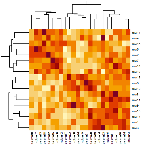
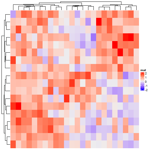
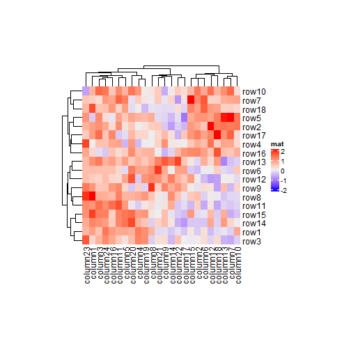
Heatmap()函数是绘制热图的基本函数,它会绘制一个热图主体,行名,列名,聚类树和注释。默认的颜色是黄色系的。
library(ComplexHeatmap)
## 载入需要的程辑包:grid
## ========================================
## ComplexHeatmap version 2.8.0
## Bioconductor page: http://bioconductor.org/packages/ComplexHeatmap/
## Github page: https://github.com/jokergoo/ComplexHeatmap
## Documentation: http://jokergoo.github.io/ComplexHeatmap-reference
##
## If you use it in published research, please cite:
## Gu, Z. Complex heatmaps reveal patterns and correlations in multidimensional
##   genomic data. Bioinformatics 2016.
##
## The new InteractiveComplexHeatmap package can directly export static
## complex heatmaps into an interactive Shiny app with zero effort. Have a try!
##
## This message can be suppressed by:
##   suppressPackageStartupMessages(library(ComplexHeatmap))
## ========================================
heatmap(mat)
2.1 颜色
对于热图可视化,颜色是数据矩阵的主要表示形式。在大多数情况下,热图用于可视化连续数值矩阵。在这种情况下,用户应提供颜色映射功能。颜色映射函数接受数值型向量,并返回对应的颜色向量。用户应始终使用circlize::colorRamp2()函数在Heatmap()中生成颜色映射。colorRamp2()的两个参数是离散型数值向量和对应的颜色向量。colorRamp2()通过LAB颜色空间在每个间隔内线性插值颜色。另外,使用colorRamp2()有助于生成带有适当刻度线的图例。
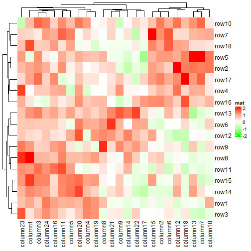
在以下示例中,线性插值-2和2之间的值以获得相应的颜色,大于2的值都映射为红色,小于-2的值都映射为绿色。
library(circlize)
## ========================================
## circlize version 0.4.13
## CRAN page: https://cran.r-project.org/package=circlize
## Github page: https://github.com/jokergoo/circlize
## Documentation: https://jokergoo.github.io/circlize_book/book/
##
## If you use it in published research, please cite:
## Gu, Z. circlize implements and enhances circular visualization
##   in R. Bioinformatics 2014.
##
## This message can be suppressed by:
##   suppressPackageStartupMessages(library(circlize))
## ========================================
col_fun = colorRamp2(c(-2, 0, 2), c("green", "white", "red"))
col_fun(seq(-3, 3))
## [1] "#00FF00FF" "#00FF00FF" "#B1FF9AFF" "#FFFFFFFF" "#FF9E81FF" "#FF0000FF"
## [7] "#FF0000FF"
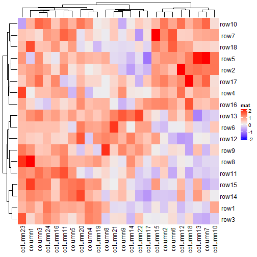
Heatmap(mat, name = "mat", col = col_fun)
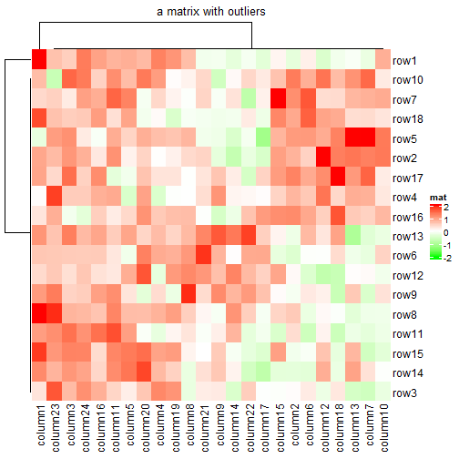
使用colorRamp2()可以精确控制颜色映射范围,并且不会受到极端值的影响。
mat2 = mat
mat2[1, 1] = 100000
Heatmap(mat2, name = "mat", col = col_fun,
    column_title = "a matrix with outliers")
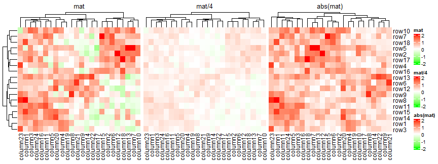
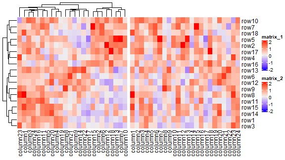
另外,使用colorRamp2()可以使得多个热图之间的颜色具有可比性,如下所示,在3个热图中,相同的颜色总是对应相同的数值:
p1 <- Heatmap(mat, name = "mat", col = col_fun, column_title = "mat")
p2 <- Heatmap(mat/4, name = "mat/4", col = col_fun, column_title = "mat/4")
p3 <- Heatmap(abs(mat), name = "abs(mat)", col = col_fun, column_title = "abs(mat)")
p1 + p2 + p3
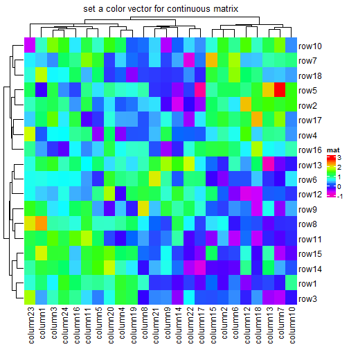
如果矩阵是连续的,也可以简单地提供颜色的向量,并且颜色将被线性插值。 但是此方法对异常值不友好,因为映射总是从矩阵中的最小值开始,以最大值结束。
Heatmap(mat, name = "mat", col = rev(rainbow(10)), column_title = "set a color vector for continuous matrix")
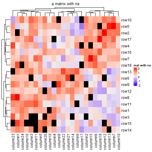
还可以可视化NA,使用na_col = "xxx"指定NA的颜色:
mat_with_na = mat
na_index = sample(c(TRUE, FALSE), nrow(mat)*ncol(mat), replace = TRUE, prob = c(1, 9))
mat_with_na[na_index] = NA
Heatmap(mat_with_na, name = "mat with na", na_col = "black", column_title = "a matrix with na")
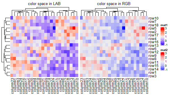
改变colorRamp2()函数的线性插值
f1 = colorRamp2(seq(min(mat), max(mat), length = 3), c("blue", "#EEEEEE", "red"))
f2 = colorRamp2(seq(min(mat), max(mat), length = 3), c("blue", "#EEEEEE", "red"), space = "RGB")

p1 <- Heatmap(mat, name = "mat1", col = f1, column_title = "color space in LAB")
p2 <- Heatmap(mat, name = "mat2", col = f2, column_title = "color space in RGB")
p1 + p2
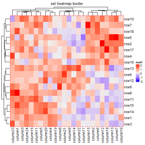
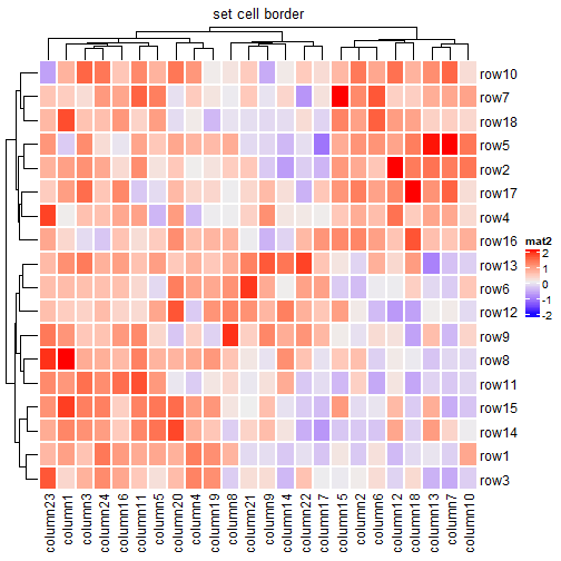
热图边框的样式通过border_gp函数控制,热图每个小格子的样式由rect_gp = gpar()函数控制。
Heatmap(mat, name = "mat1", border_gp = gpar(lty = 2, col = "red"), column_title = "set heatmap border")
Heatmap(mat, name = "mat2", column_title = "set cell border", rect_gp = gpar(col = "white", lty = 1, lwd = 2))
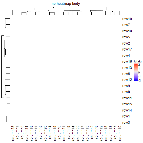
如果设置type = "none",热图主体部分不会画任何东西,可以通过cell_fun和layer_fun自定义,后面会介绍。
Heatmap(mat, name = "lalala", rect_gp = gpar(type="none"), column_title = "no heatmap body")
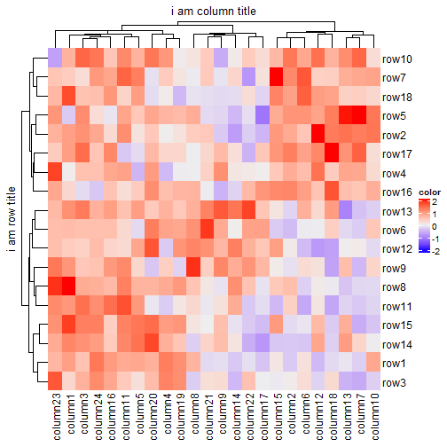
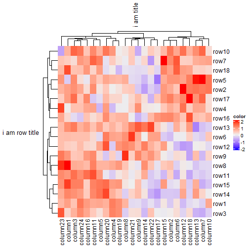
2.2 行标题/列标题
添加行标题和列标题:
Heatmap(mat, name = "color", column_title = "i am column title", row_title = "i am row title")
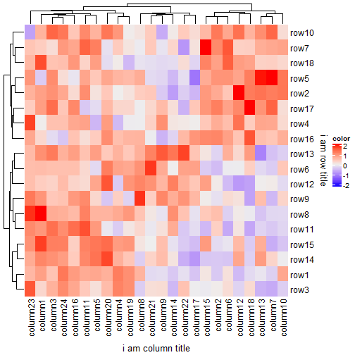
更改标题位置:
Heatmap(mat, name = "color", column_title = "i am column title", row_title = "i am row title", column_title_side = "bottom", row_title_side = "right")
旋转行/列标题:
Heatmap(mat, name = "color", column_title = "i am title", column_title_rot = 90, row_title = "i am row title", row_title_rot = 0)
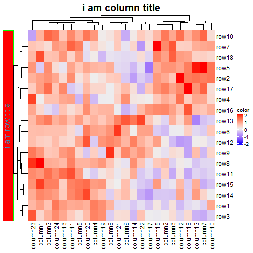
更改行/列标题样式:
Heatmap(mat, name = "color", column_title = "i am column title", row_title = "i am row title",
        column_title_gp = gpar(fontsize = 20, fontface = "bold"),
        row_title_gp = gpar(col = "steelblue", fontsize = 16, fill = "red", border = "green")
        )
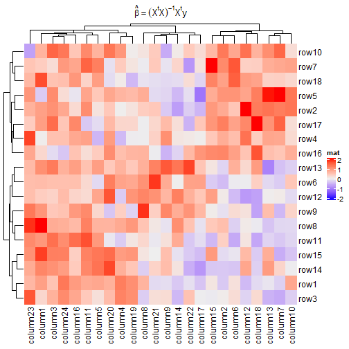
标题是公式:
Heatmap(mat, name = "mat",
    column_title = expression(hat(beta) == (X^t * X)^{-1} * X^t * y))
2.3 聚类
支持各种自定义
关闭聚类(不聚类):
p1 <- Heatmap(mat)
p2 <- Heatmap(mat, cluster_rows = F, cluster_columns = F)
p1 + p2
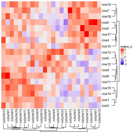
聚类但是不显示聚类树:
Heatmap(mat, show_row_dend = T, show_column_dend = F)
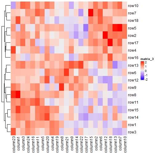
调整聚类树的位置:
Heatmap(mat, row_dend_side = "right", column_dend_side = "bottom")
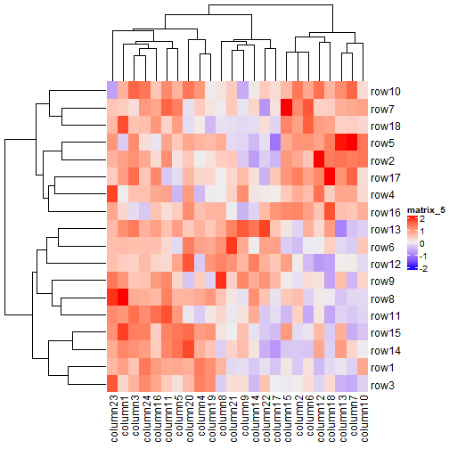
调整聚类树的高度和宽度:
Heatmap(mat, row_dend_width = unit(4, "cm"), column_dend_height = unit(3, "cm"))
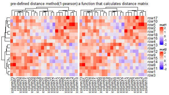
2.3.1 距离计算方法
支持:
-
pearson,spearson,kendall,三选一; -
自定义距离计算函数
p1 <- Heatmap(mat, name = "mat1", clustering_distance_rows = "pearson",
    column_title = "pre-defined distance method(1-pearson)")
p2 <- Heatmap(mat, name = "mat2", clustering_distance_rows = function(m) dist(m),
    column_title = "a function that calculates distance matrix")
p1 + p2
2.3.2 聚类方法
支持hclust函数提供的方法
Heatmap(mat, name = "mat", clustering_method_rows = "single")
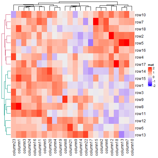
2.3.3 自定义聚类树颜色
可以借助dendextend包自定义聚类树的颜色,具体做法如下:
library(dendextend)
##
## ---------------------
## Welcome to dendextend version 1.15.1
## Type citation('dendextend') for how to cite the package.
##
## Type browseVignettes(package = 'dendextend') for the package vignette.
## The github page is: https://github.com/talgalili/dendextend/
##
## Suggestions and bug-reports can be submitted at: https://github.com/talgalili/dendextend/issues
## Or contact: <tal.galili@gmail.com>
##
## 	To suppress this message use:  suppressPackageStartupMessages(library(dendextend))
## ---------------------
##
## 载入程辑包:'dendextend'
## The following object is masked from 'package:stats':
##
##     cutree
row_dend = as.dendrogram(hclust(dist(mat)))
row_dend = color_branches(row_dend, k = 2) # `color_branches()` returns a dendrogram object
Heatmap(mat, name = "mat", cluster_rows = row_dend)
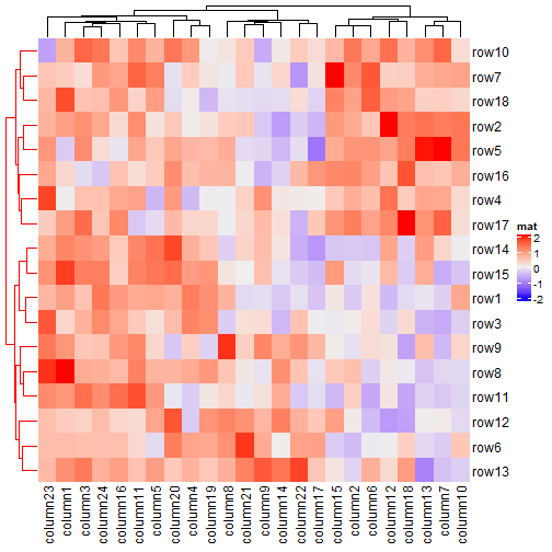
row_dend_gp和column_dend_gp参数控制聚类树样式,使用此参数会覆盖row_dend和column_dend:
Heatmap(mat, name = "mat", cluster_rows = row_dend, row_dend_gp = gpar(col = "red"))
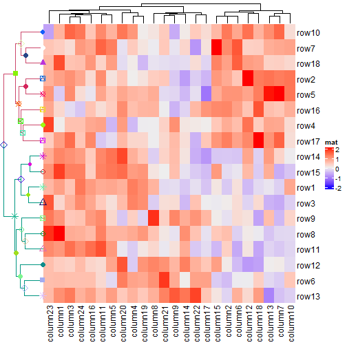
从2.5.6版本以后,可以通过提供合适的nodePar给树的节点使用不同的形状:
row_dend = dendrapply(row_dend, function(d) {
    attr(d, "nodePar") = list(cex = 0.8, pch = sample(20, 1), col = rand_color(1))
    return(d)
})
Heatmap(mat, name = "mat", cluster_rows = row_dend, row_dend_width = unit(2, "cm"))
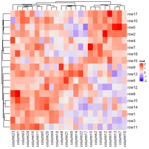
2.3.4 重新排列聚类树
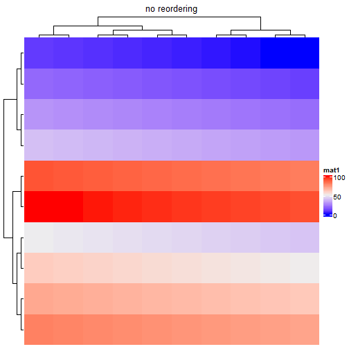
在Heatmap()函数中,对聚类树进行重新排序,以使具有较大差异的行/列彼此分离(请参阅reorder.dendrogram()文档)。 此处的差异(或称权重)是通过行/列的均值来计算的。如果将其设置为逻辑值,则row_dend_reorder和column_dend_reorder控制是否应用聚类树重排序。 如果将两个参数设置为数值向量,则它们还控制重排序的权重(会被传递给reorder.dendrogram()的wts参数)。可以通过设置row_dend_reorder = F来关闭重新排序。
默认情况下,如果将cluster_rows/cluster_columns设置为逻辑值或聚类函数,聚类树会重新排序。 如果将cluster_rows/cluster_columns设置为聚类对象,则会关闭重排序。
m2 = matrix(1:100, nr = 10, byrow = TRUE)
Heatmap(m2, name = "mat1", row_dend_reorder = FALSE, column_title = "no reordering")
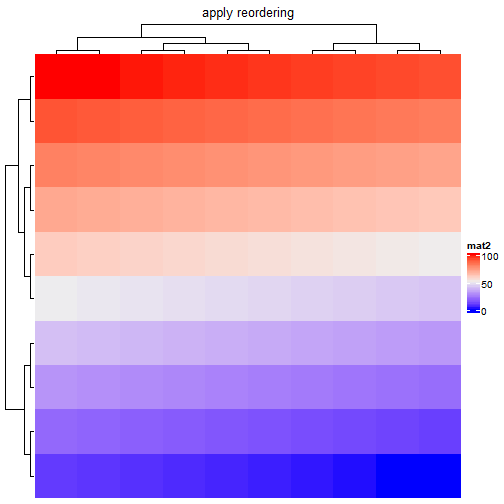
Heatmap(m2, name = "mat2", row_dend_reorder = TRUE, column_title = "apply reordering")
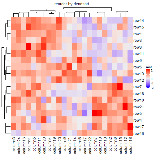
还有非常多重新排序聚类树的方法,可以使用使用dendsort包,所有的重新排序的方法都是返回排列好的聚类树对象,因此我们可以先生成排列好的行/列聚类树对象,然后再传递给cluster_rows和cluster_columns参数。
Heatmap(mat, name = "mat", column_title = "default reordering")

library(dendsort)
row_dend = dendsort(hclust(dist(mat)))
col_dend = dendsort(hclust(dist(t(mat))))
Heatmap(mat, name = "mat", cluster_rows = row_dend, cluster_columns = col_dend,
    column_title = "reorder by dendsort")
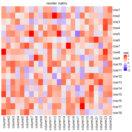
2.4 改变行/列顺序
聚类可以改变行/列顺序,我们也可以通过row_order和column_order手动改变行/列顺序
Heatmap(mat, name = "mat", row_order = order(as.numeric(gsub("row", "", rownames(mat)))),
    column_order = order(as.numeric(gsub("column", "", colnames(mat)))),
    column_title = "reorder matrix")
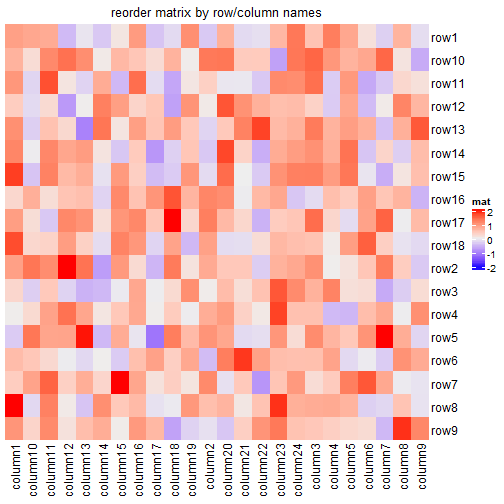
Heatmap(mat, name = "mat", row_order = sort(rownames(mat)),
    column_order = sort(colnames(mat)),
    column_title = "reorder matrix by row/column names")
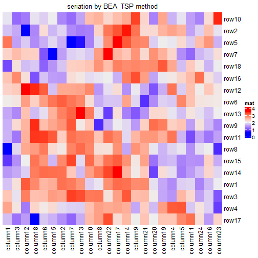
2.5 Seriation包排序
Seriation包是专门用来排序的,(详见: Make Patterns Pop Out of Heatmaps with Seriation),一些用法如下:
library(seriation)
o = seriate(max(mat) - mat, method = "BEA_TSP")
Heatmap(max(mat) - mat, name = "mat",
    row_order = get_order(o, 1), column_order = get_order(o, 2),
    column_title = "seriation by BEA_TSP method")
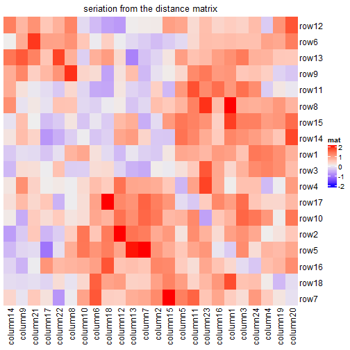
o1 = seriate(dist(mat), method = "TSP")
o2 = seriate(dist(t(mat)), method = "TSP")
Heatmap(mat, name = "mat", row_order = get_order(o1), column_order = get_order(o2),
    column_title = "seriation from the distance matrix")
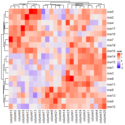
o1 = seriate(dist(mat), method = "GW")
## Registered S3 method overwritten by 'gclus':
##   method         from
##   reorder.hclust seriation
o2 = seriate(dist(t(mat)), method = "GW")

Heatmap(mat, name = "mat", cluster_rows = as.dendrogram(o1[[1]]),
    cluster_columns = as.dendrogram(o2[[1]]))
2.6 行名/列名
默认显示,如果不想显示行名/列名,使用show_row_names和show_column_names参数
Heatmap(mat, name = "mat", show_row_names = F, show_column_names = F)
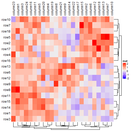
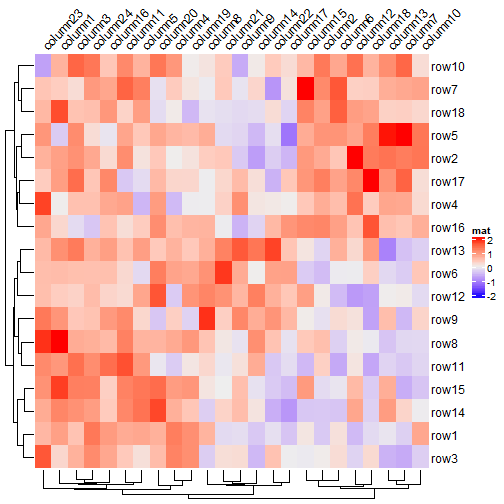
调整位置,使用row_names_side和column_names_side:
Heatmap(mat, name = "mat", row_names_side = "left", row_dend_side = "right",
    column_names_side = "top", column_dend_side = "bottom")
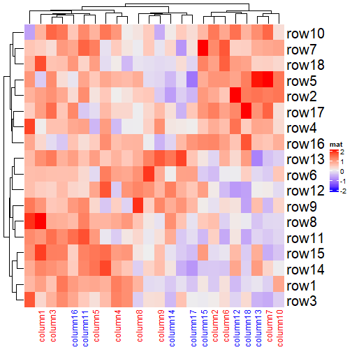
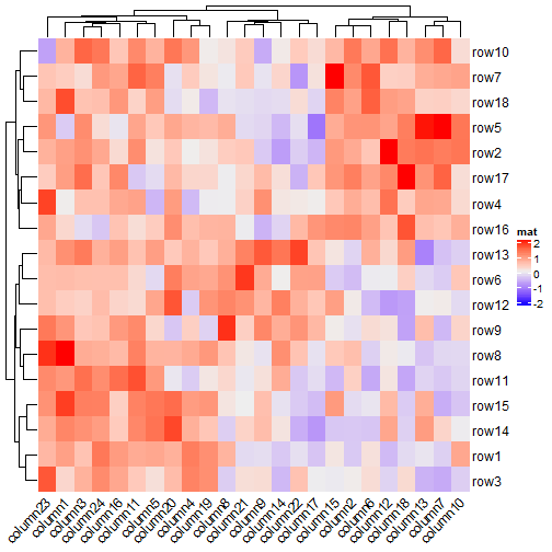
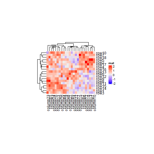
调整行名/列名样式,使用row_names_gp和column_names_gp:
Heatmap(mat, name = "mat", row_names_gp = gpar(fontsize = 20), column_names_gp = gpar(col = c(rep("red", 10), rep("blue", 8))))
居中对齐:
Heatmap(mat, name = "mat", row_names_centered = TRUE, column_names_centered = TRUE)
旋转方向:
Heatmap(mat, name = "mat", column_names_rot = 45)
Heatmap(mat, name = "mat", column_names_rot = 45, column_names_side = "top",
    column_dend_side = "bottom")
行名/列名太长怎么办?也能调整:
mat2 = mat
rownames(mat2)[1] = paste(c(letters, LETTERS), collapse = "")
Heatmap(mat2, name = "mat", row_title = "default row_names_max_width")
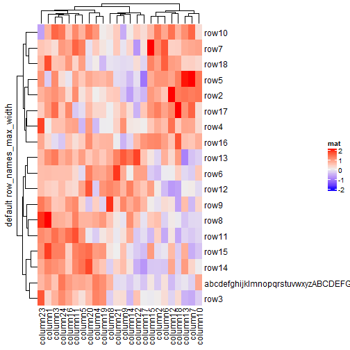
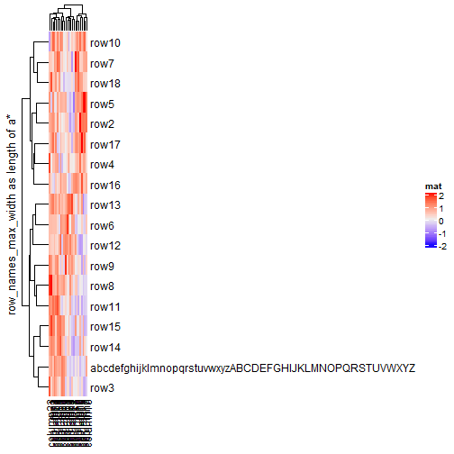
Heatmap(mat2, name = "mat", row_title = "row_names_max_width as length of a*",
    row_names_max_width = max_text_width(
        rownames(mat2),
        gp = gpar(fontsize = 12)
    ))
自定义行名/列名,可用于解决原始矩阵行名/列名不能有重复的问题,或使用特殊符号等:
# use a named vector to make sure the correspondance between row names and row labels is correct
row_labels = structure(paste0(letters[1:24], 1:24), names = paste0("row", 1:24))
column_labels = structure(paste0(LETTERS[1:24], 1:24), names = paste0("column", 1:24))
row_labels
##  row1  row2  row3  row4  row5  row6  row7  row8  row9 row10 row11 row12 row13
##  "a1"  "b2"  "c3"  "d4"  "e5"  "f6"  "g7"  "h8"  "i9" "j10" "k11" "l12" "m13"
## row14 row15 row16 row17 row18 row19 row20 row21 row22 row23 row24
## "n14" "o15" "p16" "q17" "r18" "s19" "t20" "u21" "v22" "w23" "x24"
Heatmap(mat, name = "mat", row_labels = row_labels[rownames(mat)],
    column_labels = column_labels[colnames(mat)])
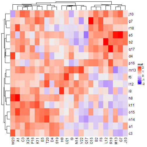
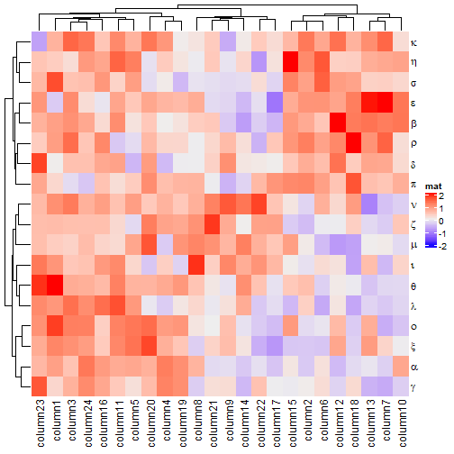
Heatmap(mat, name = "mat", row_labels = expression(alpha, beta, gamma, delta, epsilon,
    zeta, eta, theta, iota, kappa, lambda, mu, nu, xi, omicron, pi, rho, sigma))
2.7 热图分割
主要通过四个参数调整:
-
row_km -
row_split -
column_km -
column_split
2.7.1 通过K-means方法分割
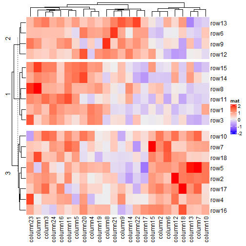
Heatmap(mat, name = "mat", row_km = 2)
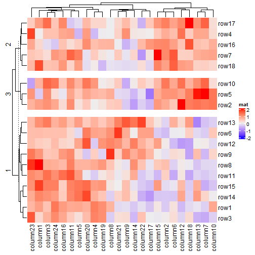
Heatmap(mat, name = "mat", column_km = 3)
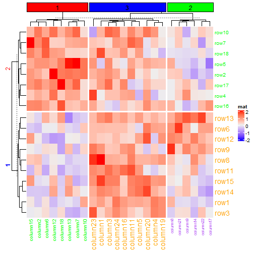
Heatmap(mat, name = "mat", row_km = 2, column_km = 3)

2.7.2 通过离散型变量分割
# split by a vector
Heatmap(mat, name = "mat",
    row_split = rep(c("A", "B"), 9), column_split = rep(c("C", "D"), 12))
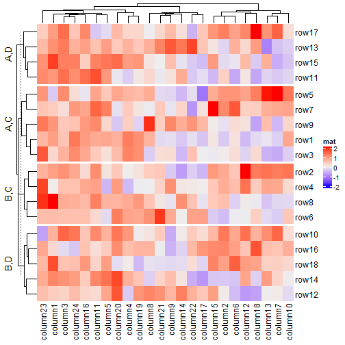
# split by a data frame
Heatmap(mat, name = "mat",
    row_split = data.frame(rep(c("A", "B"), 9), rep(c("C", "D"), each = 9)))
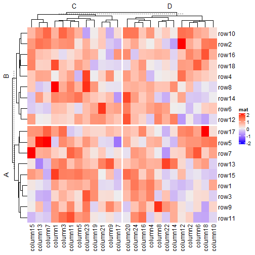
# split on both dimensions
Heatmap(mat, name = "mat", row_split = factor(rep(c("A", "B"), 9)),
    column_split = factor(rep(c("C", "D"), 12)))

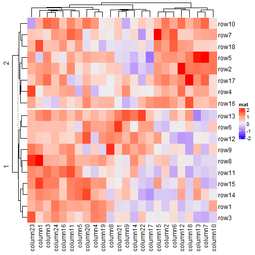
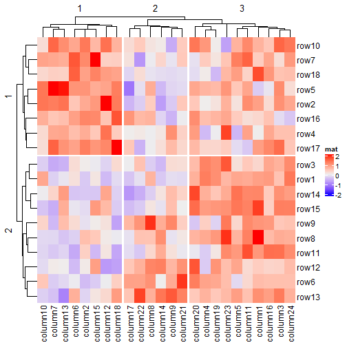
2.7.3 通过聚类树分割
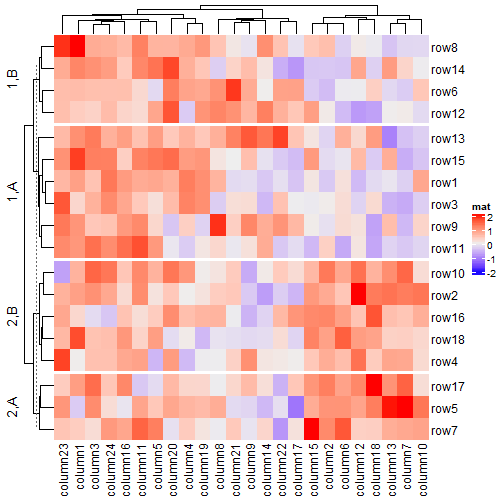
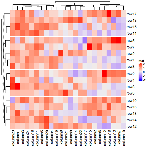
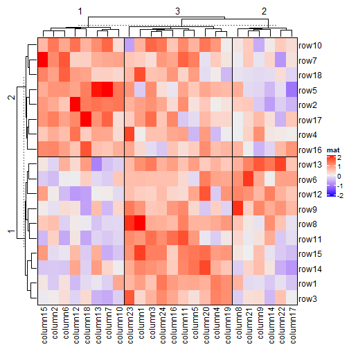
Heatmap(mat, name = "mat", row_split = 2, column_split = 3)
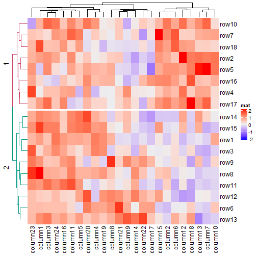
dend = hclust(dist(mat))
dend = color_branches(dend, k = 2)
Heatmap(mat, name = "mat", cluster_rows = dend, row_split = 2)
split = data.frame(cutree(hclust(dist(mat)), k = 2), rep(c("A", "B"), 9))
Heatmap(mat, name = "mat", row_split = split)
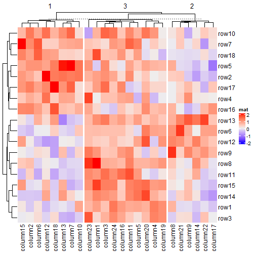
2.7.4 切片顺序
默认情况下,当把row_split/column_split设置为类别变量(向量或数据框)或设置row_km/column_km时,会对切片的平均值使用聚类,以显示切片级别中的层次结构。 在这种情况下,无法精确地控制切片的顺序,因为它是由切片的聚类控制的。但是可以将cluster_row_slices或cluster_column_slices设置为FALSE以关闭切片聚类,然后就可以精确地控制切片的顺序了。
如果没有切片聚类,则可以通过row_split/column_split中的每个变量的级别来控制每个切片的顺序(在这种情况下,每个变量应该是一个因子)。 如果所有变量都是字符,则默认顺序为unique(row_split)或unique(column_split)。
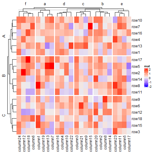
Heatmap(mat, name = "mat",
  row_split = rep(LETTERS[1:3], 6),
    column_split = rep(letters[1:6], 4))
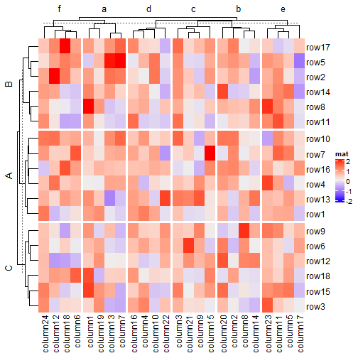
# clustering is similar as previous heatmap with branches in some nodes in the dendrogram flipped
Heatmap(mat, name = "mat",
  row_split = factor(rep(LETTERS[1:3], 6), levels = LETTERS[3:1]),
    column_split = factor(rep(letters[1:6], 4), levels = letters[6:1]))
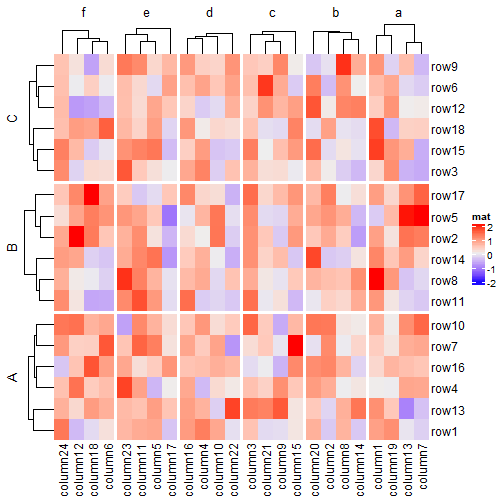
# now the order is exactly what we set
Heatmap(mat, name = "mat",
  row_split = factor(rep(LETTERS[1:3], 6), levels = LETTERS[3:1]),
    column_split = factor(rep(letters[1:6], 4), levels = letters[6:1]),
    cluster_row_slices = FALSE,
    cluster_column_slices = FALSE)
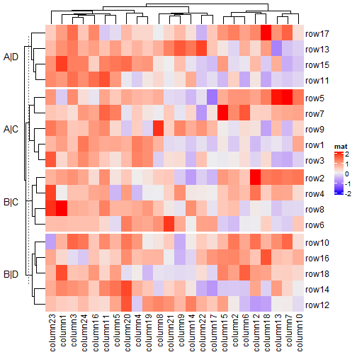
2.7.5 分割标题
split = data.frame(rep(c("A", "B"), 9), rep(c("C", "D"), each = 9))
Heatmap(mat, name = "mat", row_split = split, row_title = "%s|%s")

map = c("A" = "aaa", "B" = "bbb", "C" = "333", "D" = "444")
Heatmap(mat, name = "mat", row_split = split, row_title = "@{map[ x[1] ]}|@{map[ x[2] ]}")

Heatmap(mat, name = "mat", row_split = split, row_title = "{map[ x[1] ]}|{map[ x[2] ]}")

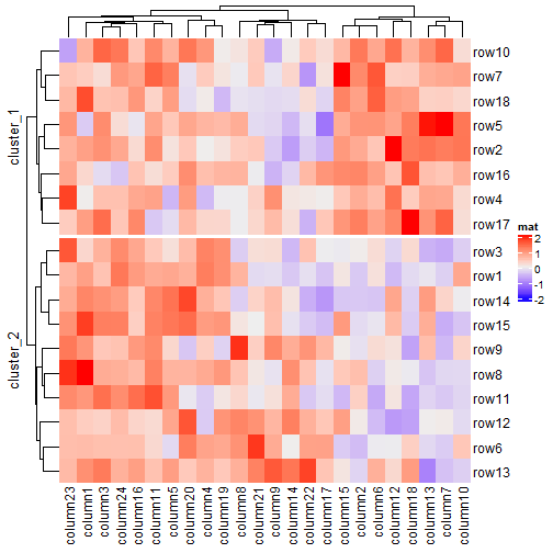
Heatmap(mat, name = "mat", row_split = split, row_title = "%s|%s", row_title_rot = 0)
Heatmap(mat, name = "mat", row_split = 2, row_title = "cluster_%s")
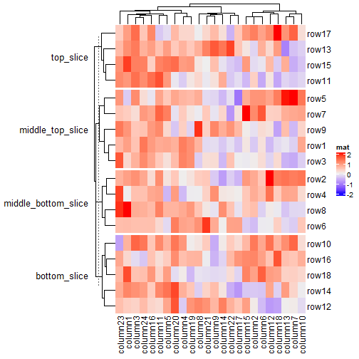
Heatmap(mat, name = "mat", row_split = split,
    row_title = c("top_slice", "middle_top_slice", "middle_bottom_slice", "bottom_slice"),
    row_title_rot = 0)
Heatmap(mat, name = "mat", row_split = split, row_title = "there are four slices")

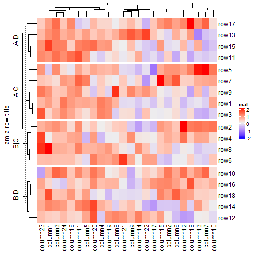
ht = Heatmap(mat, name = "mat", row_split = split, row_title = "%s|%s")
# This row_title is actually a heatmap-list-level row title
draw(ht, row_title = "I am a row title")
Heatmap(mat, name = "mat", row_split = split, row_title = NULL)
2.7.6 分割的图形参数
# 默认情况下标题顶部没有空间,现在我们增加4pt的空间
ht_opt$TITLE_PADDING = unit(c(4, 4), "points")
Heatmap(mat, name = "mat",
    row_km = 2, row_title_gp = gpar(col = c("red", "blue"), font = 1:2),
    row_names_gp = gpar(col = c("green", "orange"), fontsize = c(10, 14)),
    column_km = 3, column_title_gp = gpar(fill = c("red", "blue", "green"), font = 1:3),
    column_names_gp = gpar(col = c("green", "orange", "purple"), fontsize = c(10, 14, 8)))
2.7.7 分割宽度
Heatmap(mat, name = "mat", row_km = 3, row_gap = unit(5, "mm"))
Heatmap(mat, name = "mat", row_km = 3, row_gap = unit(c(2, 4), "mm"))
Heatmap(mat, name = "mat", row_km = 2, column_km = 3, border = TRUE)

Heatmap(mat, name = "mat", row_km = 2, column_km = 3,
    row_gap = unit(0, "mm"), column_gap = unit(0, "mm"), border = TRUE)
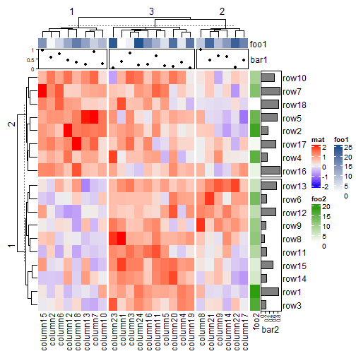
2.7.8 分割注释条
Heatmap(mat, name = "mat", row_km = 2, column_km = 3,
    top_annotation = HeatmapAnnotation(foo1 = 1:24, bar1 = anno_points(runif(24))),
    right_annotation = rowAnnotation(foo2 = 18:1, bar2 = anno_barplot(runif(18)))
)
2.8 光栅图(略)
2.9 自定义热图主体
2.9.1 cell_fun
用来调整每一个小格子,需要提供一个函数,函数共有7个参数(参数名字可以不同,但是顺序必须一样):
-
i: 行索引
-
j: 列索引
-
x: 小格子中心点横坐标
-
y: 小格子中心点纵坐标
-
width: 小格子宽度
-
height: 小格子高度
-
fill: 小格子填充色
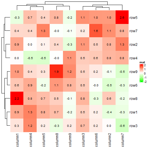
最常见的用法是在热图中添加数字:
small_mat = mat[1:9, 1:9]
col_fun = colorRamp2(c(-2, 0, 2), c("green", "white", "red"))
Heatmap(small_mat, name = "mat", col = col_fun,
    cell_fun = function(j, i, x, y, width, height, fill) {
        grid.text(sprintf("%.1f", small_mat[i, j]), x, y, gp = gpar(fontsize = 10))
})
也可以选择只添加大于0的数字:
Heatmap(small_mat, name = "mat",  col = col_fun,
    cell_fun = function(j, i, x, y, width, height, fill) {
        if(small_mat[i, j] > 0)
            grid.text(sprintf("%.1f", small_mat[i, j]), x, y, gp = gpar(fontsize = 10))
})

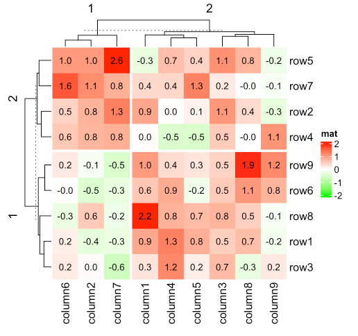
直接分割热图,无需对cell_fun()做啥:
Heatmap(small_mat, name = "mat", col = col_fun,
    row_km = 2, column_km = 2,
    cell_fun = function(j, i, x, y, width, height, fill) {
        grid.text(sprintf("%.1f", small_mat[i, j]), x, y, gp = gpar(fontsize = 10))
})
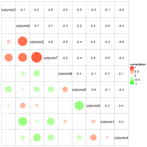
可视化相关性矩阵:
cor_mat = cor(small_mat)
od = hclust(dist(cor_mat))$order
cor_mat = cor_mat[od, od]
nm = rownames(cor_mat)
col_fun = circlize::colorRamp2(c(-1, 0, 1), c("green", "white", "red"))
# `col = col_fun` here is used to generate the legend
Heatmap(cor_mat, name = "correlation", col = col_fun, rect_gp = gpar(type = "none"),
    cell_fun = function(j, i, x, y, width, height, fill) {
        grid.rect(x = x, y = y, width = width, height = height,
            gp = gpar(col = "grey", fill = NA))
        if(i == j) {
            grid.text(nm[i], x = x, y = y)
        } else if(i > j) {
            grid.circle(x = x, y = y, r = abs(cor_mat[i, j])/2 * min(unit.c(width, height)),
                gp = gpar(fill = col_fun(cor_mat[i, j]), col = NA))
        } else {
            grid.text(sprintf("%.1f", cor_mat[i, j]), x, y, gp = gpar(fontsize = 10))
        }
    }, cluster_rows = FALSE, cluster_columns = FALSE,
    show_row_names = FALSE, show_column_names = FALSE)
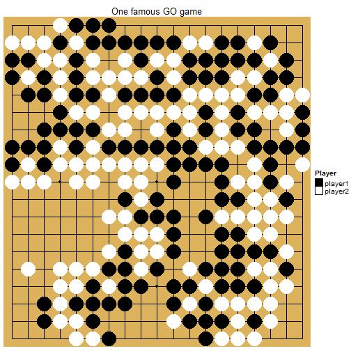
画一个棋盘:
str = "B[cp];W[pq];B[dc];W[qd];B[eq];W[od];B[de];W[jc];B[qk];W[qn]
;B[qh];W[ck];B[ci];W[cn];B[hc];W[je];B[jq];W[df];B[ee];W[cf]
;B[ei];W[bc];B[ce];W[be];B[bd];W[cd];B[bf];W[ad];B[bg];W[cc]
;B[eb];W[db];B[ec];W[lq];B[nq];W[jp];B[iq];W[kq];B[pp];W[op]
;B[po];W[oq];B[rp];W[ql];B[oo];W[no];B[pl];W[pm];B[np];W[qq]
;B[om];W[ol];B[pk];W[qp];B[on];W[rm];B[mo];W[nr];B[rl];W[rk]
;B[qm];W[dp];B[dq];W[ql];B[or];W[mp];B[nn];W[mq];B[qm];W[bp]
;B[co];W[ql];B[no];W[pr];B[qm];W[dd];B[pn];W[ed];B[bo];W[eg]
;B[ef];W[dg];B[ge];W[gh];B[gf];W[gg];B[ek];W[ig];B[fd];W[en]
;B[bn];W[ip];B[dm];W[ff];B[cb];W[fe];B[hp];W[ho];B[hq];W[el]
;B[dl];W[fk];B[ej];W[fp];B[go];W[hn];B[fo];W[em];B[dn];W[eo]
;B[gp];W[ib];B[gc];W[pg];B[qg];W[ng];B[qc];W[re];B[pf];W[of]
;B[rc];W[ob];B[ph];W[qo];B[rn];W[mi];B[og];W[oe];B[qe];W[rd]
;B[rf];W[pd];B[gm];W[gl];B[fm];W[fl];B[lj];W[mj];B[lk];W[ro]
;B[hl];W[hk];B[ik];W[dk];B[bi];W[di];B[dj];W[dh];B[hj];W[gj]
;B[li];W[lh];B[kh];W[lg];B[jn];W[do];B[cl];W[ij];B[gk];W[bl]
;B[cm];W[hk];B[jk];W[lo];B[hi];W[hm];B[gk];W[bm];B[cn];W[hk]
;B[il];W[cq];B[bq];W[ii];B[sm];W[jo];B[kn];W[fq];B[ep];W[cj]
;B[bk];W[er];B[cr];W[gr];B[gk];W[fj];B[ko];W[kp];B[hr];W[jr]
;B[nh];W[mh];B[mk];W[bb];B[da];W[jh];B[ic];W[id];B[hb];W[jb]
;B[oj];W[fn];B[fs];W[fr];B[gs];W[es];B[hs];W[gn];B[kr];W[is]
;B[dr];W[fi];B[bj];W[hd];B[gd];W[ln];B[lm];W[oi];B[oh];W[ni]
;B[pi];W[ki];B[kj];W[ji];B[so];W[rq];B[if];W[jf];B[hh];W[hf]
;B[he];W[ie];B[hg];W[ba];B[ca];W[sp];B[im];W[sn];B[rm];W[pe]
;B[qf];W[if];B[hk];W[nj];B[nk];W[lr];B[mn];W[af];B[ag];W[ch]
;B[bh];W[lp];B[ia];W[ja];B[ha];W[sf];B[sg];W[se];B[eh];W[fh]
;B[in];W[ih];B[ae];W[so];B[af]"

str = gsub("\\n", "", str)
step = strsplit(str, ";")[[1]]
type = gsub("(B|W).*", "\\1", step)
row = gsub("(B|W)\\[(.).\\]", "\\2", step)
column = gsub("(B|W)\\[.(.)\\]", "\\2", step)

go_mat = matrix(nrow = 19, ncol = 19)
rownames(go_mat) = letters[1:19]
colnames(go_mat) = letters[1:19]
for(i in seq_along(row)) {
    go_mat[row[i], column[i]] = type[i]
}
go_mat[1:4, 1:4]
##   a   b   c   d
## a NA  NA  NA  "W"
## b "W" "W" "W" "B"
## c "B" "B" "W" "W"
## d "B" "W" "B" "W"
Heatmap(go_mat, name = "go", rect_gp = gpar(type = "none"),
    cell_fun = function(j, i, x, y, w, h, col) {
        grid.rect(x, y, w, h, gp = gpar(fill = "#dcb35c", col = NA))
        if(i == 1) {
            grid.segments(x, y-h*0.5, x, y)
        } else if(i == nrow(go_mat)) {
            grid.segments(x, y, x, y+h*0.5)
        } else {
            grid.segments(x, y-h*0.5, x, y+h*0.5)
        }
        if(j == 1) {
            grid.segments(x, y, x+w*0.5, y)
        } else if(j == ncol(go_mat)) {
            grid.segments(x-w*0.5, y, x, y)
        } else {
            grid.segments(x-w*0.5, y, x+w*0.5, y)
        }

        if(i %in% c(4, 10, 16) & j %in% c(4, 10, 16)) {
            grid.points(x, y, pch = 16, size = unit(2, "mm"))
        }

        r = min(unit.c(w, h))*0.45
        if(is.na(go_mat[i, j])) {
        } else if(go_mat[i, j] == "W") {
            grid.circle(x, y, r, gp = gpar(fill = "white", col = "white"))
        } else if(go_mat[i, j] == "B") {
            grid.circle(x, y, r, gp = gpar(fill = "black", col = "black"))
        }
    },
    col = c("B" = "black", "W" = "white"),
    show_row_names = FALSE, show_column_names = FALSE,
    column_title = "One famous GO game",
    heatmap_legend_param = list(title = "Player", at = c("B", "W"),
        labels = c("player1", "player2"), border = "black")
)
2.9.2 layer_fun
用法差不多,layer_fun其实是cell_fun的“向量化版本”,速度更快,但其实作用是一样的,学会一个就可以,都会更好。
# code only for demonstration
Heatmap(..., layer_fun = function(j, i, x, y, w, h, fill) {...})
# or you can capitalize the arguments to mark they are vectors,
# the names of the argumetn do not matter
Heatmap(..., layer_fun = function(J, I, X, Y, W, H, F) {...})
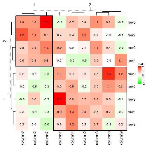
col_fun = colorRamp2(c(-2, 0, 2), c("green", "white", "red"))
Heatmap(small_mat, name = "mat", col = col_fun,
    layer_fun = function(j, i, x, y, width, height, fill) {
        # since grid.text can also be vectorized
        grid.text(sprintf("%.1f", pindex(small_mat, i, j)), x, y, gp = gpar(fontsize = 10))
})

Heatmap(small_mat, name = "mat", col = col_fun,
    row_km = 2, column_km = 2,
    layer_fun = function(j, i, x, y, width, height, fill) {
        v = pindex(small_mat, i, j)
        grid.text(sprintf("%.1f", v), x, y, gp = gpar(fontsize = 10))
        if(sum(v > 0)/length(v) > 0.75) {
            grid.rect(gp = gpar(lwd = 2, fill = "transparent"))
        }
})
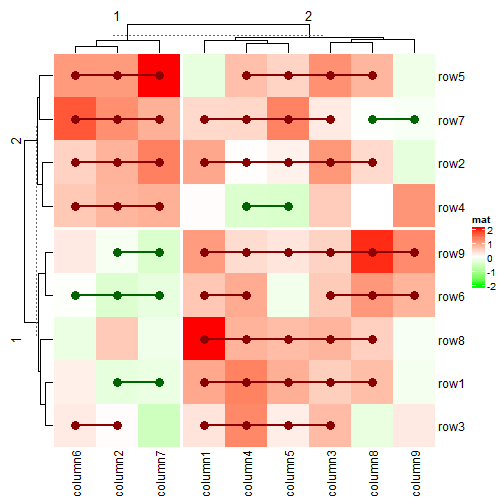
Heatmap(small_mat, name = "mat", col = col_fun,
    row_km = 2, column_km = 2,
    layer_fun = function(j, i, x, y, w, h, fill) {
        # restore_matrix() is explained after this chunk of code
        ind_mat = restore_matrix(j, i, x, y)
        for(ir in seq_len(nrow(ind_mat))) {
            # start from the second column
            for(ic in seq_len(ncol(ind_mat))[-1]) {
                ind1 = ind_mat[ir, ic-1] # previous column
                ind2 = ind_mat[ir, ic]   # current column
                v1 = small_mat[i[ind1], j[ind1]]
                v2 = small_mat[i[ind2], j[ind2]]
                if(v1 * v2 > 0) { # if they have the same sign
                    col = ifelse(v1 > 0, "darkred", "darkgreen")
                    grid.segments(x[ind1], y[ind1], x[ind2], y[ind2],
                        gp = gpar(col = col, lwd = 2))
                    grid.points(x[c(ind1, ind2)], y[c(ind1, ind2)],
                        pch = 16, gp = gpar(col = col), size = unit(4, "mm"))
                }
            }
        }
    }
)
2.10 热图大小
heatmap_width和heatmap_height控制整个热图的大小(包括图例),width和height只控制热图主体的大小
Heatmap(mat, name = "mat", width = unit(8, "cm"), height = unit(8, "cm"))
Heatmap(mat, name = "mat", heatmap_width = unit(8, "cm"), heatmap_height = unit(8, "cm"))
sessionInfo()
## R version 4.1.0 (2021-05-18)
## Platform: x86_64-w64-mingw32/x64 (64-bit)
## Running under: Windows 10 x64 (build 19044)
##
## Matrix products: default
##
## locale:
## [1] LC_COLLATE=Chinese (Simplified)_China.936
## [2] LC_CTYPE=Chinese (Simplified)_China.936
## [3] LC_MONETARY=Chinese (Simplified)_China.936
## [4] LC_NUMERIC=C
## [5] LC_TIME=Chinese (Simplified)_China.936
##
## attached base packages:
## [1] grid      stats     graphics  grDevices utils     datasets  methods
## [8] base
##
## other attached packages:
## [1] seriation_1.3.0      dendsort_0.3.4       dendextend_1.15.1
## [4] circlize_0.4.13      ComplexHeatmap_2.8.0
##
## loaded via a namespace (and not attached):
##  [1] shape_1.4.6         GetoptLong_1.0.5    tidyselect_1.1.1
##  [4] xfun_0.25           purrr_0.3.4         colorspace_2.0-2
##  [7] vctrs_0.3.8         generics_0.1.0      viridisLite_0.4.0
## [10] stats4_4.1.0        utf8_1.2.2          rlang_0.4.11
## [13] pillar_1.6.2        glue_1.4.2          DBI_1.1.1
## [16] BiocGenerics_0.38.0 RColorBrewer_1.1-2  registry_0.5-1
## [19] matrixStats_0.60.0  foreach_1.5.1       lifecycle_1.0.0
## [22] stringr_1.4.0       munsell_0.5.0       gtable_0.3.0
## [25] GlobalOptions_0.1.2 codetools_0.2-18    evaluate_0.14
## [28] knitr_1.33          IRanges_2.26.0      Cairo_1.5-12.2
## [31] doParallel_1.0.16   parallel_4.1.0      fansi_0.5.0
## [34] highr_0.9           Rcpp_1.0.7          scales_1.1.1
## [37] S4Vectors_0.30.0    magick_2.7.3        gridExtra_2.3
## [40] rjson_0.2.20        ggplot2_3.3.5       png_0.1-7
## [43] digest_0.6.27       gclus_1.3.2         stringi_1.7.3
## [46] dplyr_1.0.7         clue_0.3-59         tools_4.1.0
## [49] magrittr_2.0.1      tibble_3.1.3        cluster_2.1.2
## [52] crayon_1.4.1        pkgconfig_2.0.3     ellipsis_0.3.2
## [55] viridis_0.6.1       assertthat_0.2.1    iterators_1.0.13
## [58] TSP_1.1-10          R6_2.5.1            compiler_4.1.0
获取更多R语言和生信知识,请关注公众号:医学和生信笔记。
公众号后台回复R语言,即可获得海量学习资料!


 261
261

 被折叠的 条评论
为什么被折叠?
被折叠的 条评论
为什么被折叠?
 到【灌水乐园】发言


