【深度学习实战】p3 Pytorch实现天气识别

最新推荐文章于 2024-07-25 23:06:58 发布

Banana0840

最新推荐文章于 2024-07-25 23:06:58 发布

阅读量922

点赞数 18

文章标签：深度学习 pytorch 人工智能

本文链接：https://blog.csdn.net/Banana0840/article/details/137976474

版权

🍨 本文为🔗365天深度学习训练营中的学习记录博客
🍖 原作者：K同学啊

代码

import torch
import numpy as np
import torch.nn as nn
import torchvision.transforms as transforms
import torchvision
from torchvision import transforms, datasets

import os, PIL, pathlib, random

device = torch.device("cuda" if torch.cuda.is_available() else "cpu")

device

device(type=‘cuda’)

data_dir = './data/weather_photos/'
data_dir = pathlib.Path(data_dir)

data_paths = list(data_dir.glob('*'))
classeNames = [str(path).split("\\")[2] for path in data_paths]
classeNames

[‘cloudy’, ‘rain’, ‘shine’, ‘sunrise’]

import matplotlib.pyplot as plt
from PIL import Image

# 指定图像文件夹路径
image_folder = './data/weather_photos/cloudy/'

# 获取文件夹中的所有图像文件
image_files = [f for f in os.listdir(image_folder) if f.endswith((".jpg", ".png", ".jpeg"))]

# 创建Matplotlib图像
fig, axes = plt.subplots(1, 8, figsize=(16, 6))

# 使用列表推导式加载和显示图像
for ax, img_file in zip(axes.flat, image_files):
    img_path = os.path.join(image_folder, img_file)
    img = Image.open(img_path)
    ax.imshow(img)
    ax.axis('off')

# 显示图像
plt.tight_layout()
plt.show()

在这里插入图片描述

total_datadir = './data/weather_photos/'

# 关于transforms.Compose的更多介绍可以参考：https://blog.csdn.net/qq_38251616/article/details/124878863
train_transforms = transforms.Compose([
    transforms.Resize([224, 224]),  # 将输入图片resize成统一尺寸
    transforms.ToTensor(),          # 将PIL Image或numpy.ndarray转换为tensor，并归一化到[0,1]之间
    transforms.Normalize(           # 标准化处理-->转换为标准正太分布（高斯分布），使模型更容易收敛
        mean=[0.485, 0.456, 0.406], 
        std=[0.229, 0.224, 0.225])  # 其中 mean=[0.485,0.456,0.406]与std=[0.229,0.224,0.225] 从数据集中随机抽样计算得到的。
])

total_data = datasets.ImageFolder(total_datadir,transform=train_transforms)
total_data

Dataset ImageFolder
Number of datapoints: 1125
Root location: ./data/weather_photos/
StandardTransform
Transform: Compose(
Resize(size=[224, 224], interpolation=bilinear, max_size=None, antialias=None)
ToTensor()
Normalize(mean=[0.485, 0.456, 0.406], std=[0.229, 0.224, 0.225])
)

train_size = int(0.8 * len(total_data))
test_size  = len(total_data) - train_size
train_dataset, test_dataset = torch.utils.data.random_split(total_data, [train_size, test_size])
train_dataset, test_dataset

(<torch.utils.data.dataset.Subset at 0x17ec3b94310>,
<torch.utils.data.dataset.Subset at 0x17ebf7b5910>)

train_size,test_size

(900, 225)

batch_size = 32

train_dl = torch.utils.data.DataLoader(train_dataset,
                                       batch_size=batch_size,
                                       shuffle=True,
                                       num_workers=1)
test_dl = torch.utils.data.DataLoader(test_dataset,
                                      batch_size=batch_size,
                                      shuffle=True,
                                      num_workers=1)

for X, y in test_dl:
    print("Shape of X [N, C, H, W]: ", X.shape)
    print("Shape of y: ", y.shape, y.dtype)
    break

Shape of X [N, C, H, W]: torch.Size([32, 3, 224, 224])
Shape of y: torch.Size([32]) torch.int64

import torch.nn.functional as F

class Network_bn(nn.Module):
    def __init__(self):
        super(Network_bn, self).__init__()
        """
        nn.Conv2d()函数：
        第一个参数（in_channels）是输入的channel数量
        第二个参数（out_channels）是输出的channel数量
        第三个参数（kernel_size）是卷积核大小
        第四个参数（stride）是步长，默认为1
        第五个参数（padding）是填充大小，默认为0
        """
        self.conv1 = nn.Conv2d(in_channels=3, out_channels=12, kernel_size=5, stride=1, padding=0)
        self.bn1 = nn.BatchNorm2d(12)
        self.conv2 = nn.Conv2d(in_channels=12, out_channels=12, kernel_size=5, stride=1, padding=0)
        self.bn2 = nn.BatchNorm2d(12)
        self.pool = nn.MaxPool2d(2,2)
        self.conv4 = nn.Conv2d(in_channels=12, out_channels=24, kernel_size=5, stride=1, padding=0)
        self.bn4 = nn.BatchNorm2d(24)
        self.conv5 = nn.Conv2d(in_channels=24, out_channels=24, kernel_size=5, stride=1, padding=0)
        self.bn5 = nn.BatchNorm2d(24)
        self.fc1 = nn.Linear(24*50*50, len(classeNames))

    def forward(self, x):
        x = F.relu(self.bn1(self.conv1(x)))      
        x = F.relu(self.bn2(self.conv2(x)))     
        x = self.pool(x)                        
        x = F.relu(self.bn4(self.conv4(x)))     
        x = F.relu(self.bn5(self.conv5(x)))  
        x = self.pool(x)                        
        x = x.view(-1, 24*50*50)
        x = self.fc1(x)

        return x

device = "cuda" if torch.cuda.is_available() else "cpu"
print("Using {} device".format(device))

model = Network_bn().to(device)
model

Using cuda device
Network_bn(
(conv1): Conv2d(3, 12, kernel_size=(5, 5), stride=(1, 1))
(bn1): BatchNorm2d(12, eps=1e-05, momentum=0.1, affine=True, track_running_stats=True)
(conv2): Conv2d(12, 12, kernel_size=(5, 5), stride=(1, 1))
(bn2): BatchNorm2d(12, eps=1e-05, momentum=0.1, affine=True, track_running_stats=True)
(pool): MaxPool2d(kernel_size=2, stride=2, padding=0, dilation=1, ceil_mode=False)
(conv4): Conv2d(12, 24, kernel_size=(5, 5), stride=(1, 1))
(bn4): BatchNorm2d(24, eps=1e-05, momentum=0.1, affine=True, track_running_stats=True)
(conv5): Conv2d(24, 24, kernel_size=(5, 5), stride=(1, 1))
(bn5): BatchNorm2d(24, eps=1e-05, momentum=0.1, affine=True, track_running_stats=True)
(fc1): Linear(in_features=60000, out_features=4, bias=True)
)

loss_fn    = nn.CrossEntropyLoss() # 创建损失函数
learn_rate = 1e-5 # 学习率
opt        = torch.optim.Adam(model.parameters(),lr=learn_rate)

from torch.optim.lr_scheduler import LambdaLR

lr_lambda = lambda epoch: 1.0 if epoch < 100 else np.exp(0.1 * (10 - epoch))
scheduler = LambdaLR(opt, lr_lambda, last_epoch=-1)

# 训练循环
def train(dataloader, model, loss_fn, optimizer):
    size = len(dataloader.dataset)  # 训练集的大小，一共60000张图片
    num_batches = len(dataloader)   # 批次数目，1875（60000/32）

    train_loss, train_acc = 0, 0  # 初始化训练损失和正确率
    
    for X, y in dataloader:  # 获取图片及其标签
        X, y = X.to(device), y.to(device)
        
        # 计算预测误差
        pred = model(X)          # 网络输出
        loss = loss_fn(pred, y)  # 计算网络输出和真实值之间的差距，targets为真实值，计算二者差值即为损失
        
        # 反向传播
        optimizer.zero_grad()  # grad属性归零
        loss.backward()        # 反向传播
        optimizer.step()       # 每一步自动更新
        
        # 记录acc与loss
        train_acc  += (pred.argmax(1) == y).type(torch.float).sum().item()
        train_loss += loss.item()
            
    train_acc  /= size
    train_loss /= num_batches

    return train_acc, train_loss

def test (dataloader, model, loss_fn):
    size        = len(dataloader.dataset)  # 测试集的大小，一共10000张图片
    num_batches = len(dataloader)          # 批次数目，313（10000/32=312.5，向上取整）
    test_loss, test_acc = 0, 0
    
    # 当不进行训练时，停止梯度更新，节省计算内存消耗
    with torch.no_grad():
        for imgs, target in dataloader:
            imgs, target = imgs.to(device), target.to(device)
            
            # 计算loss
            target_pred = model(imgs)
            loss        = loss_fn(target_pred, target)
            
            test_loss += loss.item()
            test_acc  += (target_pred.argmax(1) == target).type(torch.float).sum().item()

    test_acc  /= size
    test_loss /= num_batches

    return test_acc, test_loss

epochs     = 50
train_loss = []
train_acc  = []
test_loss  = []
test_acc   = []


def scheduler_lr(optimizer, scheduler):
    lr_history = []

    """optimizer的更新在scheduler更新的前面"""
    for epoch in range(epochs):
        optimizer.step() # 更新参数
        lr_history.append(optimizer.param_groups[0]['lr'])
        # print(optimizer.param_groups[0]['lr'])
        scheduler.step() # 调整学习率
    return lr_history

lr_history = scheduler_lr(opt, scheduler)
print(lr_history)

for epoch in range(epochs):
    model.train()
    epoch_train_acc, epoch_train_loss = train(train_dl, model, loss_fn, opt)
    
    model.eval()
    epoch_test_acc, epoch_test_loss = test(test_dl, model, loss_fn)
    
    train_acc.append(epoch_train_acc)
    train_loss.append(epoch_train_loss)
    test_acc.append(epoch_test_acc)
    test_loss.append(epoch_test_loss)
    
    template = ('Epoch:{:2d}, Train_acc:{:.1f}%, Train_loss:{:.3f}, Test_acc:{:.1f}%，Test_loss:{:.3f}')
    print(template.format(epoch+1, epoch_train_acc*100, epoch_train_loss, epoch_test_acc*100, epoch_test_loss))
print('Done')

import matplotlib.pyplot as plt
#隐藏警告
import warnings
warnings.filterwarnings("ignore")               #忽略警告信息
plt.rcParams['font.sans-serif']    = ['SimHei'] # 用来正常显示中文标签
plt.rcParams['axes.unicode_minus'] = False      # 用来正常显示负号
plt.rcParams['figure.dpi']         = 100        #分辨率

epochs_range = range(epochs)

plt.figure(figsize=(12, 3))
plt.subplot(1, 3, 1)

plt.plot(epochs_range, train_acc, label='Training Accuracy')
plt.plot(epochs_range, test_acc, label='Test Accuracy')
plt.legend(loc='lower right')
plt.title('Training and Validation Accuracy')

plt.subplot(1, 3, 2)
plt.plot(epochs_range, train_loss, label='Training Loss')
plt.plot(epochs_range, test_loss, label='Test Loss')
plt.legend(loc='upper right')
plt.title('Training and Validation Loss')

plt.subplot(1, 3, 3)
plt.plot(epochs_range, lr_history, label='Learning Rate')
plt.legend(loc='upper right')
plt.title('lr')


plt.show()

本地图片预测

# 1.保存模型
 
# torch.save(model, 'model.pth') # 保存整个模型
torch.save(model.state_dict(), 'model_state_dict.pth') # 仅保存状态字典
 
# 2. 加载模型 or 新建模型加载状态字典
 
# model2 = torch.load('model.pth') 
# model2 = model2.to(device) # 理论上在哪里保存模型，加载模型也会优先在哪里，但是指定一下确保不会出错
 
model2 = Network_bn().to(device) # 重新定义模型
model2.load_state_dict(torch.load('model_state_dict.pth')) # 加载状态字典到模型
 
# 3.图片预处理
from PIL import Image
import torchvision.transforms as transforms
 
# 输入图片预处理
def preprocess_image(image_path):
    image = Image.open(image_path)
    transform = transforms.Compose([
        transforms.Resize((224, 224)),  # 假设使用的是224x224的输入
        transforms.ToTensor(),
        transforms.Normalize(mean=[0.485, 0.456, 0.406], std=[0.229, 0.224, 0.225]),
    ])
    image = transform(image).unsqueeze(0)  # 增加一个批次维度
    return image
 
# 4.预测函数（指定路径）
def predict(image_path, model):
    model.eval()  # 将模型设置为评估模式
    with torch.no_grad():  # 关闭梯度计算
        image = preprocess_image(image_path)
        image = image.to(device)  # 确保图片在正确的设备上
        outputs = model(image)
        _, predicted = torch.max(outputs, 1)  # 获取最可能的预测类别
        return predicted.item()
 
# 5.预测并输出结果
image_path = "./data/weather_photos/test.jpg"  # 替换为你的图片路径
prediction = predict(image_path, model)
class_names = ["cloudy", "rain", "shine", "sunrise"]  # Replace with your class labels
predicted_label = class_names[prediction]
print("Predicted class:", predicted_label)

Predicted class: cloudy

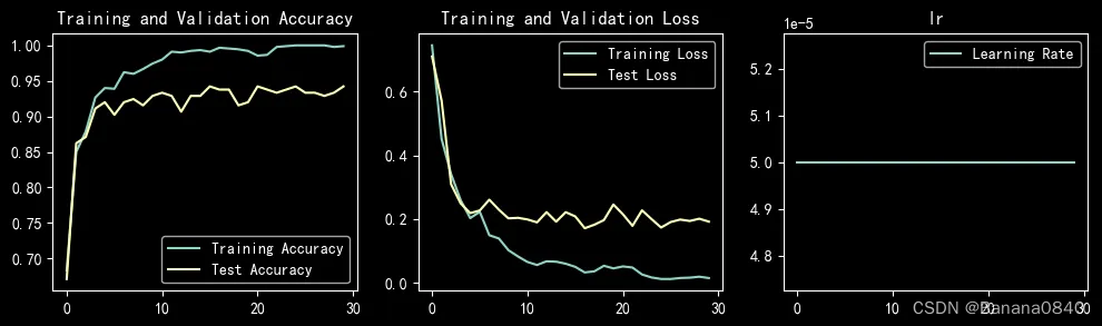
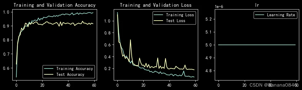
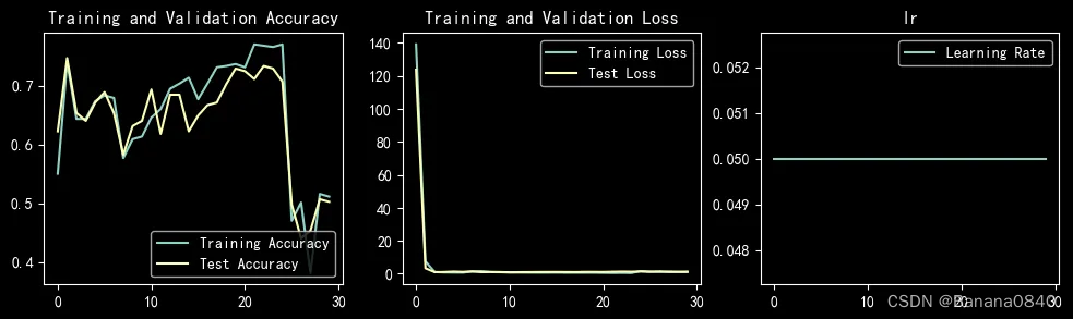
训练结果

learn_rate = 5e-05 epochs=30 SGD

在这里插入图片描述

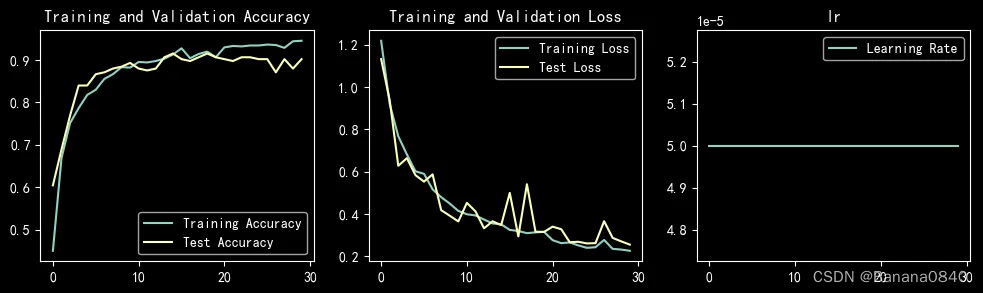
learn_rate = 5e-05 epochs=30 Adam

在这里插入图片描述

learn_rate = 5e-06 epochs=30 SGD

在这里插入图片描述

learn_rate = 5e-06 恒定学习率 epochs=30 Adam

在这里插入图片描述

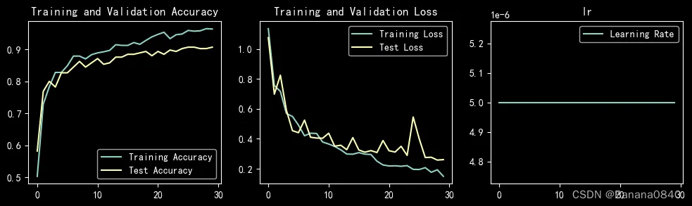
learn_rate = 5e-06 epochs=60 Adam

在这里插入图片描述

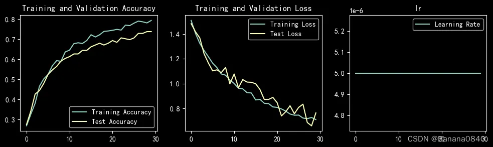
learn_rate = 5e-04 epochs=30 SGD

在这里插入图片描述

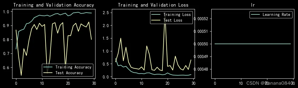
learn_rate = 5e-04 epochs=30 Adam

在这里插入图片描述

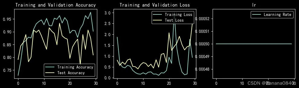
learn_rate = 5e-02 epochs=30 Adam

在这里插入图片描述

learn_rate = 1e-05 epochs=30 SGD

在这里插入图片描述

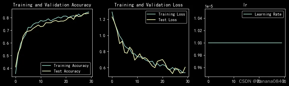
learn_rate = 1e-05 epochs=30 Adam

在这里插入图片描述

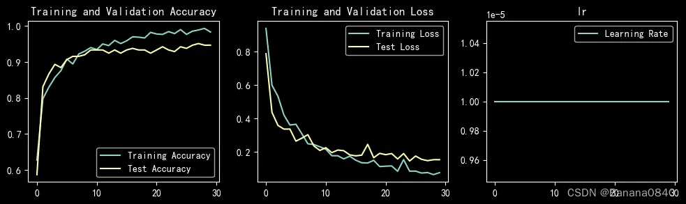
Epoch: 1, Train_acc:62.7%, Train_loss:0.940, Test_acc:58.7%，Test_loss:0.788
Epoch: 2, Train_acc:79.8%, Train_loss:0.599, Test_acc:83.1%，Test_loss:0.437
Epoch: 3, Train_acc:83.0%, Train_loss:0.533, Test_acc:86.7%，Test_loss:0.359
Epoch: 4, Train_acc:85.7%, Train_loss:0.421, Test_acc:89.3%，Test_loss:0.337
Epoch: 5, Train_acc:87.6%, Train_loss:0.361, Test_acc:88.4%，Test_loss:0.337
Epoch: 6, Train_acc:90.8%, Train_loss:0.366, Test_acc:90.7%，Test_loss:0.264
Epoch: 7, Train_acc:89.4%, Train_loss:0.309, Test_acc:91.6%，Test_loss:0.282
Epoch: 8, Train_acc:92.2%, Train_loss:0.249, Test_acc:91.6%，Test_loss:0.303
Epoch: 9, Train_acc:93.0%, Train_loss:0.244, Test_acc:92.0%，Test_loss:0.236
Epoch:10, Train_acc:94.0%, Train_loss:0.231, Test_acc:93.3%，Test_loss:0.209
Epoch:11, Train_acc:93.4%, Train_loss:0.216, Test_acc:93.3%，Test_loss:0.225
Epoch:12, Train_acc:95.0%, Train_loss:0.177, Test_acc:93.3%，Test_loss:0.196
Epoch:13, Train_acc:94.6%, Train_loss:0.177, Test_acc:92.4%，Test_loss:0.211
Epoch:14, Train_acc:96.0%, Train_loss:0.158, Test_acc:93.3%，Test_loss:0.207
Epoch:15, Train_acc:95.1%, Train_loss:0.174, Test_acc:92.4%，Test_loss:0.182
Epoch:16, Train_acc:95.9%, Train_loss:0.150, Test_acc:93.3%，Test_loss:0.176
Epoch:17, Train_acc:97.0%, Train_loss:0.135, Test_acc:93.8%，Test_loss:0.181
Epoch:18, Train_acc:96.9%, Train_loss:0.134, Test_acc:93.3%，Test_loss:0.245
Epoch:19, Train_acc:96.7%, Train_loss:0.150, Test_acc:93.3%，Test_loss:0.165
Epoch:20, Train_acc:98.2%, Train_loss:0.112, Test_acc:92.4%，Test_loss:0.191
Epoch:21, Train_acc:97.8%, Train_loss:0.114, Test_acc:93.3%，Test_loss:0.183
Epoch:22, Train_acc:97.7%, Train_loss:0.116, Test_acc:94.2%，Test_loss:0.190
Epoch:23, Train_acc:98.4%, Train_loss:0.084, Test_acc:93.3%，Test_loss:0.158
Epoch:24, Train_acc:97.9%, Train_loss:0.154, Test_acc:92.9%，Test_loss:0.190
Epoch:25, Train_acc:99.0%, Train_loss:0.085, Test_acc:94.2%，Test_loss:0.146
Epoch:26, Train_acc:97.7%, Train_loss:0.085, Test_acc:93.8%，Test_loss:0.175
Epoch:27, Train_acc:98.6%, Train_loss:0.073, Test_acc:94.7%，Test_loss:0.156
Epoch:28, Train_acc:98.9%, Train_loss:0.076, Test_acc:95.1%，Test_loss:0.148
Epoch:29, Train_acc:99.3%, Train_loss:0.064, Test_acc:94.7%，Test_loss:0.153
Epoch:30, Train_acc:98.3%, Train_loss:0.076, Test_acc:94.7%，Test_loss:0.154
Done

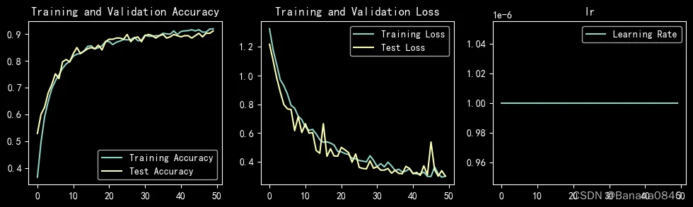
learn_rate = 1e-06 恒定学习率 epochs=50 Adam

在这里插入图片描述

learn_rate = 1e-06 恒定学习率 epochs=80 Adam

在这里插入图片描述

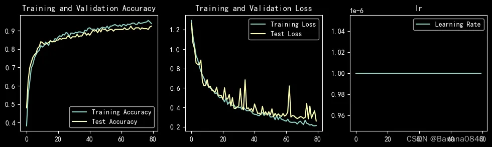
learn_rate = 1e-06 恒定学习率 epochs=80

在这里插入图片描述

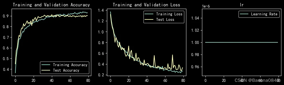
learn_rate = 1e-05 恒定学习率 epochs=50 Adam

在这里插入图片描述

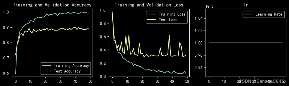
训练中准确度达到过95%的参数配置

learn_rate = 1e-05 epochs=30 Adam

结论

Adam是自适应学习率优化器，完全可以手动，但是手动比较困难，理论上来说，我认为手动应该比Adam效果会更好，只不过对于增大减小的度的把控还有待确定。
初始学习率可以设置相对大一点，但是不能过大，过大会导致拟合出现大幅度震荡

上次问题

batch_size对于test_accuracy有什么影响
本次没有测试batch_size的问题，留到后续
如何分阶段配置学习率
本次没有手动配置，留到后续
sgd、adam等不同的优化器对比
sgd：
随机梯度下降，模型的参数向负梯度方向更新，使得损失函数的值逐渐减少。具体来说，每个训练样本的误差对每个参数的偏导数被计算，并且应用于参数的当前值以更新它。在迭代过程中，每次更新后，下一个样本的误差被计算，参数再次更新。这个过程重复多次，直到达到一定的收敛条件或达到事先设定的最大迭代次数。
adam：
是一种自适应学习率的优化算法，是在动量梯度下降和自适应学习率算法的基础上发展而来的。Adam算法将不同的梯度给予不同的权重，使得神经网络在学习率稳定时，能快速、稳定的收敛到最佳点。具体来说，Adam算法维护了每个权重的一阶梯度平均值和二阶梯度平均值的指数加权移动平均数。
其实应该讨论一下这两种优化器的数学原理，看了看没太看懂。

一个框架看懂优化算法之异同 SGD/AdaGrad/Adam
优化器介绍—SGD、Adam、Adagrad