扩散模型 Diffusion Models - 原理篇

扩散模型 Diffusion Models - 原理篇

参考博客及视频链接：

What are Diffusion Models?

Diffusion Model扩散模型理论与完整PyTorch代码详细解读

论文：

2015 年 Deep Unsupervised Learning using Nonequilibrium Thermodynamics

2020 年 Generative Modeling by Estimating Gradients of the Data Distribution

2020 年 Denoising Diffusion Probabilistic Models

数学公式基础

1. 联合条件概率
   $$\begin{gathered} P(A,B,C)=P(C|A,B)P(A,B)=P(C|A,B)P(B|A)P(A) \\ P(B,C|A)=P(A,B,C)/P(A)=P(C|A,B)P(B|A) \end{gathered}$$

2. 基于马尔可夫假说的联合条件概率，如果满足 A->B->C，则
   $$\begin{gathered} P(A,B,C)=P(C|A,B)P(A,B)=P(C|B)P(B|A)P(A) \\ P(B,C|A)=P(A,B,C)/P(A)=P(C|B)P(B|A) \end{gathered}$$

3. 高斯分布的 KL 散度公式

   对于两个单一变量的高斯分布 p 和 q 而言：
   $$KL(p,q)=log\frac{{\sigma }_2}{{\sigma }_1}+\frac{{\sigma }_1^2+({\mu }_1-{\mu }_2{)}^2}{2{\sigma }_2^2}-\frac{1}{2}$$

4. 参数重采样

   为了网络可训练，从高斯分布 $\mathcal{N}(\mu ,\sigma )$ 中采样，等价于先从标准分布 $\mathcal{N}(0,I)$ 采样出 $z$ ，再得到 $\sigma \ast z+\mu$ 。

原理

扩散模型的灵感来自于非平衡热力学。定义了一个扩散步骤的马尔可夫链（当前状态只与上一时刻的状态有关），慢慢地向真实数据中添加随机噪声（前向过程），然后学习反向扩散过程（逆扩散过程），从噪声中构建所需的数据样本。

前向过程

前向过程是不含可学习参数的，随着 $t$ 不断增大，最终分布变成各向独立的高斯分布。定义真实数据分布 $x_0\sim q(x)$ ，我们在前向过程中逐步加入一个小的高斯噪声，一共加入 $T$ 步，从而产生了一系列加噪的样本 $x_1,x_2,\dots ,x_T$ ，加入噪声的均值和方差由 ${\beta }_t$ 决定，其在 $(0,1)$ 之间，且 ${\beta }_1<{\beta }_2<\cdots <{\beta }_T$ ，这意味着所加的噪声是越来越大的。
$$q(x_t|x_{t-1})=\mathcal{N}(x_t;\sqrt{1-{\beta }_t}{x}_{t-1},{\beta }_{t}I)$$
由于定义为马尔可夫链，所以给定 $x_0$ 的 $x_{1:T}$ 的联合概率分布为
$$q(x_{1:T}|x_0)={\Pi }_{t=1}^{T}q(x_t|x_{t-1})$$
上述式子计算 $q(x_t|x_0)$ 需要不断迭代，我们希望给定 $x_0,{\beta }_t$ 就可以计算出来。给定 ${\alpha }_t=1-{\beta }_t,{\bar{\alpha }}_t={\Pi }_{i=1}^t{\alpha }_i$
$$\begin{array}{rl}{x}_t& =\sqrt{{\alpha }_t}{x}_{t-1}+\sqrt{1-{\alpha }_t}{z}_{t-1}\#参数重整化和替换\\ & =\sqrt{{\alpha }_t}(\sqrt{{\alpha }_{t-1}}{x}_{t-2}+\sqrt{1-{\alpha }_{t-1}}{z}_{t-2})+\sqrt{1-{\alpha }_t}{z}_{t-1}\\ & =\sqrt{{\alpha }_t{\alpha }_{t-1}}{x}_{t-2}+\sqrt{{\alpha }_t-{\alpha }_t{\alpha }_{t-1}}{z}_{t-2}+\sqrt{1-{\alpha }_t}{z}_{t-1}\\ & \\ & \#由于两个正态分布X\sim \mathcal{N}({\mu }_1,{\sigma }_1),Y\sim \mathcal{N}({\mu }_2,{\sigma }_2)叠加后的分布aX+bY的均值是a{\mu }_1+b{\mu }_2,方差是a^2{\sigma }_1^2+b^2{\sigma }_2^2\\ & \#所以\sqrt{{\alpha }_t-{\alpha }_t{\alpha }_{t-1}}{z}_{t-2}+\sqrt{1-{\alpha }_t}{z}_{t-1}均值为0，方差为1-{\alpha }_t{\alpha }_{t-1}再利用参数重整化\\ & \\ & =\sqrt{{\alpha }_t{\alpha }_{t-1}}{x}_{t-2}+\sqrt{1-{\alpha }_t{\alpha }_{t-1}}{\bar{z}}_{t-2}\#此{\bar{z}}_{t-2}不同于z_{t-2}\\ & =\dots \\ & =\sqrt{{\bar{\alpha }}_t}{x}_0+\sqrt{1-{\bar{\alpha }}_t}z\#参数逆重整化\\ & \\ & q(x_t|x_0)=\mathcal{N}(x_t;\sqrt{{\bar{\alpha }}_t}{x}_0,(1-{\bar{\alpha }}_t)I)\#此时无需迭代即可算出任意时刻q(x_t|x_0)\end{array}$$

逆扩散过程

逆过程是从高斯噪声中恢复原始数据，由于正向过程中我们每次加的噪声很小，所以我们假设 $p(x_{t-1}|x_t)$ 也是一个高斯分布，我们可以使用神经网络进行拟合。逆过程也是一个马尔科夫链过程。
$$p_{\theta }(x_{t-1}|x_t)=\mathcal{N}(x_{t-1};{\mu }_{\theta }(x_t,t),{\Sigma }_{\theta }(x_t,t))$$

$$p_{\theta }(x_{0:T})=p(x_T){\Pi }_{t=1}^T{p}_{\theta }(x_{t-1}|x_t)$$

尽管 $p_{\theta }(x_{t-1}|x_t)$ 无法显式表示，但是 $p_{\theta }(x_{t-1}|x_t，x_0)$ 可以用公式表示: $q(x_{t-1}|x_t,x_0)=\mathcal{N}(x_{t-1};\bar{\mu }(x_t,x_0),{\bar{\beta }}_{t}I)$。求 $\bar{\mu }、{\bar{\beta }}_t$
$$\begin{array}{rl}q(x_{t-1}|x_t,x_0)& =\frac{q(x_{t-1},x_t,x_0)}{q(x_t,x_0)}\\ & =\frac{q(x_t|x_{t-1},x_0)q(x_{t-1}|x_0)q(x_0)}{q(x_t|x_0)q(x_0)}\#分子分母约掉\\ & =\frac{q(x_t|x_{t-1},x_0)q(x_{t-1}|x_0)}{q(x_t|x_0)}\#马尔科夫链假设\\ & =\frac{q(x_t|x_{t-1})q(x_{t-1}|x_0)}{q(x_t|x_0)}\#带入高斯分布概率密度函数f(x)=\frac{1}{\sqrt{2\pi }\sigma }{e}^{-\frac{(x-\mu {)}^2}{2{\sigma }^2}}\\ & \propto \exp (-\frac{1}{2}((\frac{(x_t-\sqrt{{\alpha }_t}{x}_{t-1}{)}^2}{{\beta }_t})+\frac{(x_{t-1}-\sqrt{{\bar{\alpha }}_{t-1}}{x}_0{)}^2}{1-{\bar{\alpha }}_{t-1}}-\frac{(x_t-\sqrt{{\bar{\alpha }}_t}{x}_0{)}^2}{1-{\bar{\alpha }}_t}))\#因为我们只需要估计均值和方差，写出指数项即可\\ & =\exp (-\frac{1}{2}((\frac{{\alpha }_t}{{\beta }_t}+\frac{1}{1-{\bar{\alpha }}_{t-1}})x_{t-1}^2-(\frac{2\sqrt{{\alpha }_t}}{{\beta }_t}{x}_t+\frac{2\sqrt{\overline{{\alpha }_t}}}{1-{\bar{\alpha }}_t}{x}_0)x_{t-1}+C(x_t,x_0))\#C(x_t.x_0)与x_{t-1}无关的函数，会导致有偏\\ & \\ & \#由a{x}^2+bx=\frac{(x+\frac{b}{2a}{)}^2}{\frac{1}{a}}+C，可得到均值和方差\\ & \\ {\bar{\beta }}_t=& \frac{1}{\frac{{\alpha }_t}{{\beta }_t}+\frac{1}{1-{\bar{\alpha }}_{t-1}}}=\frac{1-{\bar{\alpha }}_{t-1}}{1-{\bar{\alpha }}_t}{\beta }_t\#常数\\ \bar{\mu }(x_t,x_0)=& \frac{\frac{2\sqrt{{\alpha }_t}}{{\beta }_t}{x}_t+\frac{2\sqrt{\overline{{\alpha }_t}}}{1-{\bar{\alpha }}_t}{x}_0}{2\times (\frac{{\alpha }_t}{{\beta }_t}+\frac{1}{1-{\bar{\alpha }}_{t-1}})}=\frac{\sqrt{{\alpha }_t}(1-{\bar{\alpha }}_{t-1})}{1-{\bar{\alpha }}_t}{x}_t+\frac{\sqrt{{\bar{\alpha }}_{t-1}}{\beta }_t}{1-{\bar{\alpha }}_t}{x}_0\#与x_t和x_0有关\\ =& \frac{\sqrt{{\alpha }_t}(1-{\bar{\alpha }}_{t-1})}{1-{\bar{\alpha }}_t}{x}_t+\frac{\sqrt{{\bar{\alpha }}_{t-1}}{\beta }_t}{1-{\bar{\alpha }}_t}(\frac{1}{\sqrt{{\bar{\alpha }}_t}}(x_t-\sqrt{1-{\bar{\alpha }}_t}{z}_t))\#已知x_t的情况下，x_0可以用x_t表示，x_t=\sqrt{{\bar{\alpha }}_t}{x}_0+\sqrt{1-{\bar{\alpha }}_t}z\\ =& \frac{{\alpha }_t(1-\frac{{\bar{\alpha }}_t}{{\alpha }_t})}{{\sqrt{\alpha }}_t(1-{\bar{\alpha }}_t)}{x}_t+\frac{\sqrt{{\bar{\alpha }}_{t-1}}(1-{\alpha }_t)}{1-{\bar{\alpha }}_t}\frac{1}{\sqrt{{\alpha }_t}\sqrt{{\bar{\alpha }}_{t-1}}}(x_t-\sqrt{1-{\bar{\alpha }}_t}{z}_t)\\ =& \frac{{\alpha }_t-{\bar{\alpha }}_t+1-{\alpha }_t}{{\sqrt{\alpha }}_t(1-{\bar{\alpha }}_t)}{x}_t-\frac{1-{\alpha }_t}{\sqrt{{\alpha }_t}\sqrt{1-{\bar{\alpha }}_t}}{z}_t\\ =& \frac{1}{\sqrt{{\alpha }_t}}(x_t-\frac{{\beta }_t}{\sqrt{1-{\bar{\alpha }}_t}}{z}_t)\#尽管该式不含x_0，但是前提是给定x_0的条件下才推出此式\end{array}$$
接下来就是算目标数据分布的似然函数，这样网络才可以进行训练。
$$\begin{array}{rl}-\log p_{\theta }(x_0)& \le -\log p_{\theta }(x_0)+D_{KL}(q(x_{1:T}|x_0)||p_{\theta }(x_{1:T}|x_0))\#KL散度大于对于0\\ & =-\log p_{\theta }(x_0)+{\mathbb{E}}_{x_{1:T}\sim q(x_{1:T}|x_0)}(\log \frac{q(x_{1:T}|x_0)}{\frac{p_{\theta }(x_{0:T})}{p_{\theta }(x_0)}})\\ & =-\log p_{\theta }(x_0)+{\mathbb{E}}_{x_{1:T}\sim q(x_{1:T}|x_0)}(\log \frac{q(x_{1:T}|x_0)}{p_{\theta }(x_{0:T})}+\log p_{\theta }(x_0)\\ & \#等式两边同乘以期望{\mathbb{E}}_{q(x_0)}\\ {\mathbb{E}}_{q(x_0)}-\log p_{\theta }(x_0)& \le {\mathbb{E}}_{q(x_{0:T}|x_0)}(\log \frac{q(x_{1:T}|x_0)}{p_{\theta }(x_{0:T})}\#左侧为交叉熵，右侧为上界\\ & ={\mathbb{E}}_q(\log \frac{{\Pi }_{t=1}^{T}q(x_t|x_{t-1})}{p_{\theta }(x_T){\Pi }_{t=1}^{T}p(x_{t-1}|x_t)})\\ & ={\mathbb{E}}_q(-\log p_{\theta }(x_T)+{\Sigma }_{t=1}^T\log \frac{q(x_t|x_{t-1})}{p(x_{t-1}|x_t)})\\ & ={\mathbb{E}}_q(-\log p_{\theta }(x_T)+{\Sigma }_{t=2}^T\log \frac{q(x_t|x_{t-1})}{p(x_{t-1}|x_t)}+\log \frac{q(x_1|x_0)}{p(x_0|x_1)})\\ & ={\mathbb{E}}_q(-\log p_{\theta }(x_T)+{\Sigma }_{t=2}^T\log \frac{q(x_t|x_{t-1})}{p(x_{t-1}|x_t)}+\log \frac{q(x_1|x_0)}{p(x_0|x_1)})\\ \#& 中间一项分子q(x_t|x_{t-1})=q(x_t|x_{t-1},x_0)=\frac{q(x_t,x_{t-1},x_0)}{q(x_{t-1},x_0)}=\frac{q(x_{t-1}|x_t,x_0)q(x_t|x_0)q(x_0)}{q(x_{t-1},x_0)}=\frac{q(x_{t-1}|x_t,x_0)q(x_t|x_0)}{q(x_{t-1}|x_0)}\\ & ={\mathbb{E}}_q(-\log p_{\theta }(x_T)+{\Sigma }_{t=2}^T\log \frac{q(x_{t-1}|x_t,x_0)}{p(x_{t-1}|x_t)}+{\Sigma }_{t=2}^T\log \frac{q(x_t|x_0)}{q(x_{t-1}|x_0)}+\log \frac{q(x_1|x_0)}{p(x_0|x_1)})\\ & ={\mathbb{E}}_q(-\log p_{\theta }(x_T)+{\Sigma }_{t=2}^T\log \frac{q(x_{t-1}|x_t,x_0)}{p(x_{t-1}|x_t)}+\log \frac{q(x_T|x_0)}{q(x_1|x_0)}+\log \frac{q(x_1|x_0)}{p(x_0|x_1)})\#化简第三项\\ & ={\mathbb{E}}_q(\log \frac{q(x_T|x_0)}{p_{\theta }(x_T)}+{\Sigma }_{t=2}^T\log \frac{q(x_{t-1}|x_t,x_0)}{p(x_{t-1}|x_t)}-\log p(x_0|x_1))\#后两项化简，第三项提到第一项\\ & ={\mathbb{E}}_q(D_{KL}(q(x_T|x_0)||p_{\theta }(x_T)))+{\Sigma }_{t=2}^T{D}_{KL}(q(x_{t-1}|x_t,x_0)||p_{\theta }(x_{t-1}|x_t))-\log p(x_0|x_1))\#后两项可以合并成一项\\ & ={\mathbb{E}}_q(D_{KL}(q(x_T|x_0)||p_{\theta }(x_T)))+{\Sigma }_{t=1}^T{D}_{KL}(q(x_{t-1}|x_t,x_0)||p_{\theta }(x_{t-1}|x_t))\#第一项不含参数，p_{\theta }(x_T)是各项同性的高斯分布\end{array}$$
DDPM 论文将 $p_{\theta }(x_{t-1}|x_t)=\mathcal{N}(x_{t-1};{\mu }_{\theta }(x_t,t),{\Sigma }_{\theta }(x_t,t))$ 中的方差设置为常数 ${\beta }_t$，所以可学习的参数就只在均值中。对于两个单一变量的高斯分布p和q而言，$KL(p,q)=\log \frac{{\sigma }_2}{{\sigma }_1}+\frac{{\sigma }_1^2+({\mu }_1-{\mu }_2{)}^2}{2{\sigma }_2^2}-\frac{1}{2}$
$$\begin{gathered} 优化式子:{\Sigma }_{t=1}^T{D}_{KL}(q(x_{t-1}|x_t,x_0)||p_{\theta }(x_{t-1}|x_t)) \\ \#q为已知有偏高斯分布，p为所要拟合的分布，由于假设p方差{\sigma }_t为常数，则我们只需逼近p和q的均值即可,等价于: \\ \begin{array}{rl}最小化式子:Loss& ={\mathbb{E}}_q(\frac{1}{2{\sigma }_t^2}||{\bar{\mu }}_t(x_t,x_0)-{\mu }_{\theta }(x_t,t)|{|}^2)+C\#x_t是由x_0和噪声ϵ决定的变量\\ & ={\mathbb{E}}_{x_0,ϵ}(\frac{1}{2{\sigma }_t^2}||{\bar{\mu }}_t(x_t(x_0,ϵ),\frac{1}{\sqrt{{\bar{\alpha }}_t}}(x_t(x_0,ϵ)-\sqrt{1-\bar{\alpha }}ϵ))-{\mu }_{\theta }(x_t,t)|{|}^2)\#带入{\bar{\mu }}_t公式，上述的x_0可不做替换\\ & ={\mathbb{E}}_{x_0,ϵ}(\frac{1}{2{\sigma }_t^2}||\frac{1}{\sqrt{{\alpha }_t}}(x_t(x_0,ϵ)-\frac{{\beta }_t}{\sqrt{1-{\bar{\alpha }}_t}}ϵ)-{\mu }_{\theta }(x_t,t)|{|}^2)\\ \#& 作者认为直接预测恢复的数据效果不好，转而预测噪声，这个想法有点像预测残差连接中的残差\\ \#& 一个网络输入x_0、{\bar{\alpha }}_t、高斯噪声ϵ和t，然后预测高斯噪声ϵ\\ & ={\mathbb{E}}_{x_0,ϵ}(\frac{1}{2{\sigma }_t^2}||\frac{1}{\sqrt{{\alpha }_t}}(x_t(x_0,ϵ)-\frac{{\beta }_t}{\sqrt{1-{\bar{\alpha }}_t}}ϵ)-\frac{1}{\sqrt{{\alpha }_t}}(x_t-\frac{{\beta }_t}{\sqrt{1-{\bar{\alpha }}_t}}{ϵ}_{\theta }(x_t,t))|{|}^2)\\ & ={\mathbb{E}}_{x_0,ϵ}(\frac{{\beta }_t^2}{2{\sigma }_t^2{\alpha }_t(1-{\bar{\alpha }}_t)}||ϵ-{ϵ}_{\theta }(\sqrt{{\bar{\alpha }}_t}{x}_0+\sqrt{1-{\bar{\alpha }}_t}ϵ,t)|{|}^2)\end{array} \end{gathered}$$
作者在训练时发现，去掉 Loss 前的系数，可使训练稳定，所以简化后的 Loss 为
$$Loss={\mathbb{E}}_{x_0,ϵ}(||ϵ-{ϵ}_{\theta }(\sqrt{{\bar{\alpha }}_t}{x}_0+\sqrt{1-{\bar{\alpha }}_t}ϵ,t)|{|}^2)$$
拟合出来的均值为 ${\mu }_{\theta }(x_t,t)=\frac{1}{\sqrt{{\alpha }_t}}(x_t-\frac{{\beta }_t}{\sqrt{1-{\bar{\alpha }}_t}}{ϵ}_{\theta }(x_t,t)))$ 可用于采样。

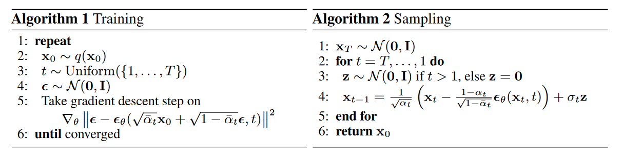
训练和采样过程

训练过程：从数据集中采样 $x_0$，从均匀分布采样 t，可使模型鲁棒，采样噪声，计算 Loss 更新模型。

采样过程：从标准正态分布采样 $x_T$ ，迭代计算 $x_{t-1}$ ，已知均值 ${\mu }_{\theta }(x_t,t)$ 和常数方差 ${\beta }_t$ 利用参数重整化可计算出 $x_{t-1}$ ，直到 $x_0$。

Pytorch 示例代码

import matplotlib.pyplot as plt
import numpy as np
from sklearn.datasets import make_moons
import torch
import torch.nn as nn
import io
from PIL import Image

moons_curve,_ = make_moons(10**4,noise=0.05)
print("shape of moons:",np.shape(moons_curve))

data = moons_curve.T

fig,ax = plt.subplots()
ax.scatter(*data,color='blue',edgecolor='white');
ax.axis('off')
dataset = torch.Tensor(moons_curve).float()

num_steps = 100             # 扩散 100 步
#制定每一步的beta
betas = torch.linspace(-6, 6, num_steps)
betas = torch.sigmoid(betas)*(0.5e-2 - 1e-5)+1e-5   # 先压缩到 0~1 再乘以 0.005

#计算alpha、alpha_prod、alpha_prod_previous、alpha_bar_sqrt等变量的值
alphas = 1-betas			
alphas_prod = torch.cumprod(alphas, 0)
alphas_prod_p = torch.cat([torch.tensor([1]).float(), alphas_prod[:-1]], 0)  #插入第一个数 1，丢掉最后一个数，previous连乘
alphas_bar_sqrt = torch.sqrt(alphas_prod)
one_minus_alphas_bar_log = torch.log(1 - alphas_prod)
one_minus_alphas_bar_sqrt = torch.sqrt(1 - alphas_prod)

assert alphas.shape == alphas_prod.shape == alphas_prod_p.shape == alphas_bar_sqrt.shape == one_minus_alphas_bar_log.shape == one_minus_alphas_bar_sqrt.shape
print("all the same shape", betas.shape)	#所有值都是同等维度，且都是常值

#计算任意时刻的x采样值，基于x_0和重参数化 前向过程
def q_x(x_0,t):
    noise = torch.randn_like(x_0)
    alphas_t = alphas_bar_sqrt[t]
    alphas_1_m_t = one_minus_alphas_bar_sqrt[t]
    return (alphas_t * x_0 + alphas_1_m_t * noise)  # 在x[0]的基础上添加噪声

num_shows = 20
fig, axs = plt.subplots(2, 10, figsize=(28, 3))
plt.rc('text', color='black')

# 共有10000个点，每个点包含两个坐标。生成100步中每隔5步加噪声后的图像,最终应该会成为一个各向同性的高斯分布
for i in range(num_shows):
    j = i // 10
    k = i % 10
    q_i = q_x(dataset, torch.tensor([i*num_steps//num_shows]))  # 生成t时刻的采样数据
    axs[j, k].scatter(q_i[:, 0], q_i[:, 1], color='red', edgecolor='white')
    axs[j, k].set_axis_off()
    axs[j, k].set_title('$q(\mathbf{x}_{'+str(i*num_steps//num_shows)+'})$')
fig.show()

class MLPDiffusion(nn.Module):					# 定义一个 MLP 模型
    def __init__(self, n_steps, num_units=128):
        super(MLPDiffusion, self).__init__()

        self.linears = nn.ModuleList(
            [
                nn.Linear(2, num_units),
                nn.ReLU(),
                nn.Linear(num_units, num_units),
                nn.ReLU(),
                nn.Linear(num_units, num_units),
                nn.ReLU(),
                nn.Linear(num_units, 2),
            ]
        )
        self.step_embeddings = nn.ModuleList(
            [
                nn.Embedding(n_steps, num_units),
                nn.Embedding(n_steps, num_units),
                nn.Embedding(n_steps, num_units),
            ]
        )

    def forward(self, x, t):
        # x = x_0
        for idx, embedding_layer in enumerate(self.step_embeddings):	# 三层
            t_embedding = embedding_layer(t)
            x = self.linears[2 * idx](x)
            x += t_embedding
            x = self.linears[2 * idx + 1](x)

        x = self.linears[-1](x)					# 输出维度与输入一致

        return x

def diffusion_loss_fn(model, x_0, alphas_bar_sqrt, one_minus_alphas_bar_sqrt, n_steps):
    """对任意时刻t进行采样计算loss"""
    batch_size = x_0.shape[0]

    # 对一个batchsize样本生成随机的时刻t
    t = torch.randint(0, n_steps, size=(batch_size // 2,))		# 为了 t 不重复，先采样一半
    t = torch.cat([t, n_steps - 1 - t], dim=0)					 
    t = t.unsqueeze(-1)

    # x0的系数
    a = alphas_bar_sqrt[t]

    # 随机噪声eps的系数
    aml = one_minus_alphas_bar_sqrt[t]

    # 生成随机噪音eps
    e = torch.randn_like(x_0)

    # 构造模型的输入
    x = x_0 * a + e * aml

    # 送入模型，得到t时刻的随机噪声预测值
    output = model(x, t.squeeze(-1))

    # 与真实噪声一起计算误差，求平均值
    return (e - output).square().mean()

def p_sample_loop(model, shape, n_steps, betas, one_minus_alphas_bar_sqrt):
    """从x[T]恢复x[T-1]、x[T-2]|...x[0]"""
    cur_x = torch.randn(shape)
    x_seq = [cur_x]
    for i in reversed(range(n_steps)):
        cur_x = p_sample(model, cur_x, i, betas, one_minus_alphas_bar_sqrt)
        x_seq.append(cur_x)
    return x_seq


def p_sample(model, x, t, betas, one_minus_alphas_bar_sqrt):
    """从 x_t 开始生成 t-1 时刻的重构值"""
    t = torch.tensor([t])

    coeff = betas[t] / one_minus_alphas_bar_sqrt[t]

    eps_theta = model(x, t)

    mean = (1 / (1 - betas[t]).sqrt()) * (x - (coeff * eps_theta))

    z = torch.randn_like(x)
    sigma_t = betas[t].sqrt()

    sample = mean + sigma_t * z

    return (sample)

# 开始训练模型
seed = 1234
print('Training model...')
batch_size = 128
dataloader = torch.utils.data.DataLoader(dataset,batch_size=batch_size,shuffle=True)
num_epoch = 4001
plt.rc('text',color='blue')

model = MLPDiffusion(num_steps)			# 输出维度是2，输入是x和step
optimizer = torch.optim.Adam(model.parameters(),lr=1e-3)

for t in range(num_epoch):
    for idx,batch_x in enumerate(dataloader):
        loss = diffusion_loss_fn(model, batch_x, alphas_bar_sqrt, one_minus_alphas_bar_sqrt, num_steps)
        optimizer.zero_grad()
        loss.backward()
        torch.nn.utils.clip_grad_norm_(model.parameters(), 1.)		# 梯度裁剪
        optimizer.step()
        
    if(t%100==0):			
        print(loss)
        x_seq = p_sample_loop(model, dataset.shape, num_steps, betas, one_minus_alphas_bar_sqrt)
        
        fig,axs = plt.subplots(1,10,figsize=(28,3))
        for i in range(1,11):
            cur_x = x_seq[i*10].detach()
            axs[i-1].scatter(cur_x[:,0], cur_x[:,1], color='red', edgecolor='white');
            axs[i-1].set_axis_off();
            axs[i-1].set_title('$q(\mathbf{x}_{'+str(i*10)+'})$')
    	fig.show()

第 0 个 epoch，100 次扩散，每 10 次输出一次

第 1000 个 epoch：

第 2000 个epoch：

第 3000 个epoch：

# 生成扩散和逆扩散的 GIF
imgs = []
for i in range(100):
    plt.clf()
    q_i = q_x(dataset,torch.tensor([i]))
    plt.scatter(q_i[:,0],q_i[:,1],color='red',edgecolor='white',s=5);
    plt.axis('off');
    
    img_buf = io.BytesIO()
    plt.savefig(img_buf,format='png')
    img = Image.open(img_buf)
    imgs.append(img)
reverse = []
for i in range(100):
    plt.clf()
    cur_x = x_seq[i].detach()
    plt.scatter(cur_x[:,0],cur_x[:,1],color='red',edgecolor='white',s=5);
    plt.axis('off')
    
    img_buf = io.BytesIO()
    plt.savefig(img_buf,format='png')
    img = Image.open(img_buf)
    reverse.append(img)
imgs = imgs + reverse
imgs[0].save("diffusion.gif", format='GIF', append_images=imgs, save_all=True, duration=100, loop=0)

总结

这是入门扩散模型的第一篇学习笔记，看到原始扩散模型还是有很多不足之处，比如 ${\beta }_t$ 如何设置更好，比如采用基于 cos 函数的变化，又如再逆扩散过程中将方差设置成一个常数，这在一定程度上抑制了模型的拟合能力。此外，在加速采样和引入条件可控的扩散是近两年研究的热点。接下来，我会继续学习这一领域的内容。