


作者:chen_h
微信号 & QQ:862251340
微信公众号:coderpai
(五)如何用 Python 从头开始实现 Bagging 算法
文本探索了众所周知的AdaBoost M1算法,该算法结合了几种弱分类器来创建更好的整体分类器。 该文包括三个主要部分:
- 回顾Adaboost M1算法及其内部工作的直观可视化
- Python中的一个实现,使用Sklearn决策树桩作为弱分类器
- 关于学习率与弱分类器参数数量之间权衡的讨论
AdaBoost 算法的直观解释
AdaBoost 回顾
假设
G
m
(
x
)
G_m(x)
Gm(x) m=1,2,3…M 是弱分类器的序列,我们的目标是构建以下内容:
G
(
x
)
=
sign
(
α
1
G
1
(
x
)
+
α
2
G
2
(
x
)
+
…
α
M
G
M
(
x
)
)
=
sign
(
∑
m
=
1
M
α
m
G
m
(
x
)
)
G(x)=\operatorname{sign}\left(\alpha_{1} G_{1}(x)+\alpha_{2} G_{2}(x)+\ldots \alpha_{M} G_{M}(x)\right)=\operatorname{sign}\left(\sum_{m=1}^{M} \alpha_{m} G_{m}(x)\right)
G(x)=sign(α1G1(x)+α2G2(x)+…αMGM(x))=sign(m=1∑MαmGm(x))
- 最终预测是通过加权多数投票来组合所有分类器的预测
- 系数 α m \alpha_m αm 由boosting算法完成,该系数对每个 G m ( x ) G_m(x) Gm(x) 进行加权。效果是对序列中更准确的分类器产生更大的影响
- 在每一个 boosting 步骤中,通过将权重 w1,w2,…,wN 应用到每个训练样本来修改数据的分布。在步骤 m,我们先将分类错误的样本的权重提高,将正确分类的样本的权重降低
- 注意,在第一步 m=1 时,权重需要平均初始化 wi = 1/N
具体算法为:
-
初始化所有的权重 w i = 1 / N w_i = 1/N wi=1/N
-
For m = 1,2,3, … ,M
-
计算加权误差:
E r r m = ∑ i − 1 N w i I ( y ( i ) ≠ G m ( x ( i ) ) ∑ i = 1 N w i E r r_{m}=\frac{\sum_{i-1}^{N} w_{i} I\left(y^{(i)} \neq G_{m}\left(x^{(i)}\right)\right.}{\sum_{i=1}^{N} w_{i}} Errm=∑i=1Nwi∑i−1NwiI(y(i)̸=Gm(x(i)) -
计算系数:
α m = log ( 1 − e r r m e r r m ) \alpha_{m}=\log \left(\frac{1-e r r_{m}}{e r r_{m}}\right) αm=log(errm1−errm) -
更新权重:
w i ← w i exp [ α m I ( y ( i ) ≠ G m ( x ( i ) ) ) ] w_{i} \leftarrow w_{i} \exp \left[\alpha_{m} \mathcal{I}\left(y^{(i)} \neq G_{m}\left(x^{(i)}\right)\right)\right] wi←wiexp[αmI(y(i)̸=Gm(x(i)))]
-
-
输出:
G ( x ) = sign [ ∑ m = 1 M α m G m ( x ) ] G(x)=\operatorname{sign}\left[\sum_{m=1}^{M} \alpha_{m} G_{m}(x)\right] G(x)=sign[m=1∑MαmGm(x)]
简单例子
假设我们使用一个如下最简单的数据集来测试我们的 AdaBoost 模型。迭代次数 M = 10,弱分类器是深度为1和2的决策树。数据是下图的红色点和蓝色点,很明显这是一个非线性的分类,但是我们的模型应该能很好地工作。

可视化弱分类器的序列模型和样本权重
前 6 个弱学习器 m =1,2,3,4,5,6 如下所示。在每次迭代时根据它们各自的样本权重来缩放散点。
第一次迭代
- 因为我们是弱分类器,所以决策边界非常简单(线性方式)
- 正如预期的那样,所有点的大小都相同
- 6个蓝点位于红色区域,并且被错误分类
第二次迭代
- 线性决策边界已经改变
- 之前错误分类的蓝色点现在更大(更大的 sample_weight)并影响了决策边界
- 9个蓝点现在被错误分类
10次迭代后的最终结果
所有分类器在不同位置具有线性决策边界。前 6 次迭代 α m \alpha_m αm 的系数为:([1.041, 0.875, 0.837, 0.781, 1.04 , 0.938…
正如预期的那样,第一次迭代具有最大的系数,因为它是错误分类最少的系数。
从头开始实现 AdaBoost M1
导入库
import matplotlib.pyplot as plt
from matplotlib.colors import ListedColormap
import numpy as np
import seaborn as sns
sns.set_style('white')

from sklearn.tree import DecisionTreeClassifier
from sklearn.ensemble import AdaBoostClassifier
数据集和适用的可视化函数
#Toy Dataset
x1 = np.array([.1,.2,.4,.8, .8, .05,.08,.12,.33,.55,.66,.77,.88,.2,.3,.4,.5,.6,.25,.3,.5,.7,.6])
x2 = np.array([.2,.65,.7,.6, .3,.1,.4,.66,.77,.65,.68,.55,.44,.1,.3,.4,.3,.15,.15,.5,.55,.2,.4])
y = np.array([1,1,1,1,1,1,1,1,1,1,1,1,1,-1,-1,-1,-1,-1,-1,-1,-1,-1,-1])
X = np.vstack((x1,x2)).T

def plot_decision_boundary(classifier, X, y, N = 10, scatter_weights = np.ones(len(y)) , ax = None ):
    '''Utility function to plot decision boundary and scatter plot of data'''
    x_min, x_max = X[:, 0].min() - .1, X[:, 0].max() + .1
    y_min, y_max = X[:, 1].min() - .1, X[:, 1].max() + .1
    xx, yy = np.meshgrid( np.linspace(x_min, x_max, N), np.linspace(y_min, y_max, N))


    #Check what methods are available
    if hasattr(classifier, "decision_function"):
        zz = np.array( [classifier.decision_function(np.array([xi,yi]).reshape(1,-1)) for  xi, yi in zip(np.ravel(xx), np.ravel(yy)) ] )
    elif hasattr(classifier, "predict_proba"):
        zz = np.array( [classifier.predict_proba(np.array([xi,yi]).reshape(1,-1))[:,1] for  xi, yi in zip(np.ravel(xx), np.ravel(yy)) ] )
    else :
        zz = np.array( [classifier(np.array([xi,yi]).reshape(1,-1)) for  xi, yi in zip(np.ravel(xx), np.ravel(yy)) ] )

    # reshape result and plot
    Z = zz.reshape(xx.shape)
    cm_bright = ListedColormap(['#FF0000', '#0000FF'])

    #Get current axis and plot
    if ax is None:
        ax = plt.gca()
    ax.contourf(xx, yy, Z, 2, cmap='RdBu', alpha=.5)
    ax.contour(xx, yy, Z,  2, cmap='RdBu')
    ax.scatter(X[:,0],X[:,1], c = y, cmap = cm_bright, s = scatter_weights * 40)
    ax.set_xlabel('$X_1$')
    ax.set_ylabel('$X_2$')
sklearn adaboost 和决策边界
boost = AdaBoostClassifier( base_estimator = DecisionTreeClassifier(max_depth = 1, max_leaf_nodes=2),
                            algorithm = 'SAMME',n_estimators=10, learning_rate=1.0)
boost.fit(X,y)
plot_decision_boundary(boost, X,y, N = 50)#, weights)
plt.show()

boost.score(X,y)
1.0

python实现
def AdaBoost_scratch(X,y, M=10, learning_rate = 1):
    #Initialization of utility variables
    N = len(y)
    estimator_list, y_predict_list, estimator_error_list, estimator_weight_list, sample_weight_list = [], [],[],[],[]

    #Initialize the sample weights
    sample_weight = np.ones(N) / N
    sample_weight_list.append(sample_weight.copy())

    #For m = 1 to M
    for m in range(M):

        #Fit a classifier
        estimator = DecisionTreeClassifier(max_depth = 1, max_leaf_nodes=2)
        estimator.fit(X, y, sample_weight=sample_weight)
        y_predict = estimator.predict(X)

        #Misclassifications
        incorrect = (y_predict != y)

        #Estimator error
        estimator_error = np.mean( np.average(incorrect, weights=sample_weight, axis=0))

        #Boost estimator weights
        estimator_weight =  learning_rate * np.log((1. - estimator_error) / estimator_error)

        #Boost sample weights
        sample_weight *= np.exp(estimator_weight * incorrect * ((sample_weight > 0) | (estimator_weight < 0)))

        #Save iteration values
        estimator_list.append(estimator)
        y_predict_list.append(y_predict.copy())
        estimator_error_list.append(estimator_error.copy())
        estimator_weight_list.append(estimator_weight.copy())
        sample_weight_list.append(sample_weight.copy())


    #Convert to np array for convenience
    estimator_list = np.asarray(estimator_list)
    y_predict_list = np.asarray(y_predict_list)
    estimator_error_list = np.asarray(estimator_error_list)
    estimator_weight_list = np.asarray(estimator_weight_list)
    sample_weight_list = np.asarray(sample_weight_list)

    #Predictions
    preds = (np.array([np.sign((y_predict_list[:,point] * estimator_weight_list).sum()) for point in range(N)]))
    print('Accuracy = ', (preds == y).sum() / N)

    return estimator_list, estimator_weight_list, sample_weight_list
运行代码
Accuracy = 100% - 结果跟 Sklearn 实现一样。
estimator_list, estimator_weight_list, sample_weight_list = AdaBoost_scratch(X,y, M=10, learning_rate = 1)
Accuracy = 1.0
adaboost_scratch 可视化
def plot_AdaBoost_scratch_boundary(estimators,estimator_weights, X, y, N = 10,ax = None ):

    def AdaBoost_scratch_classify(x_temp, est,est_weights ):
        '''Return classification prediction for a given point X and a previously fitted AdaBoost'''
        temp_pred = np.asarray( [ (e.predict(x_temp)).T* w for e, w in zip(est,est_weights )]  ) / est_weights.sum()
        return np.sign(temp_pred.sum(axis = 0))


    '''Utility function to plot decision boundary and scatter plot of data'''
    x_min, x_max = X[:, 0].min() - .1, X[:, 0].max() + .1
    y_min, y_max = X[:, 1].min() - .1, X[:, 1].max() + .1
    xx, yy = np.meshgrid( np.linspace(x_min, x_max, N), np.linspace(y_min, y_max, N))


    zz = np.array( [AdaBoost_scratch_classify(np.array([xi,yi]).reshape(1,-1), estimators,estimator_weights ) for  xi, yi in zip(np.ravel(xx), np.ravel(yy)) ] )

    # reshape result and plot
    Z = zz.reshape(xx.shape)
    cm_bright = ListedColormap(['#FF0000', '#0000FF'])

    if ax is None:
        ax = plt.gca()
    ax.contourf(xx, yy, Z, 2, cmap='RdBu', alpha=.5)
    ax.contour(xx, yy, Z,  2, cmap='RdBu')
    ax.scatter(X[:,0],X[:,1], c = y, cmap = cm_bright)
    ax.set_xlabel('$X_1$')
    ax.set_ylabel('$X_2$')
绘制决策边界
plot_AdaBoost_scratch_boundary(estimator_list, estimator_weight_list, X, y, N = 50 )

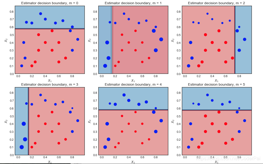
查看 AdaBoost 中弱分类器的决策边界
- M=10 迭代
- 散点的大小与 sample_weights 的比例成正比
例如,在左上图 m = 0,6个蓝色点被错误分类。在下一个方差 m = 1 中,它们的样本权重增加,散点图显示也变大。
estimator_list, estimator_weight_list, sample_weight_list  = AdaBoost_scratch(X,y, M=10, learning_rate = 1)

fig = plt.figure(figsize = (14,14))
for m in range(0,9):
    fig.add_subplot(3,3,m+1)
    s_weights = (sample_weight_list[m,:] / sample_weight_list[m,:].sum() ) * 40
    plot_decision_boundary(estimator_list[m], X,y,N = 50, scatter_weights =s_weights )
    plt.title('Estimator decision boundary, m = {}'.format(m))
Accuracy = 1.0

学习率和迭代次数之间的直观解释
这篇文章基于 AdaBoost 算法类似于 M1 或者 SAMME 实现的假设,可以按如下方式进行分类:
设
G
m
(
x
)
G_m(x)
Gm(x) m = 1,2,…,M 是弱分类器的序列,我们的目标是:
G
(
x
)
=
sign
(
α
1
G
1
(
x
)
+
α
2
G
2
(
x
)
+
…
α
M
G
M
(
x
)
)
=
sign
(
∑
m
=
1
M
α
m
G
m
(
x
)
)
G(x)=\operatorname{sign}\left(\alpha_{1} G_{1}(x)+\alpha_{2} G_{2}(x)+\ldots \alpha_{M} G_{M}(x)\right)=\operatorname{sign}\left(\sum_{m=1}^{M} \alpha_{m} G_{m}(x)\right)
G(x)=sign(α1G1(x)+α2G2(x)+…αMGM(x))=sign(m=1∑MαmGm(x))
AdaBoost M1
-
初始化权重: w i = 1 / N w_i = 1/N wi=1/N
-
For m = 1,2,3,….,M
-
计算加权误差:$ Err_m = \frac{\sum_{i-1}^N w_i \mathcal{I}(y^{(i)} \neq G_m(x^{(i)}) )}{\sum_{i=1}^N w_i}$
-
计算估算系数:
α m = L log ( 1 − e r r m e r r m ) \alpha_{m}=L \log \left(\frac{1-e r r_{m}}{e r r_{m}}\right) αm=Llog(errm1−errm)
其中, L ≤ 1 L\leq 1 L≤1 是学习率 -
更新数据权重:
w i ← w i exp [ α m I ( y ( i ) ≠ G m ( x ( i ) ) ) ] w_{i} \leftarrow w_{i} \exp \left[\alpha_{m} \mathcal{I}\left(y^{(i)} \neq G_{m}\left(x^{(i)}\right)\right)\right] wi←wiexp[αmI(y(i)̸=Gm(x(i)))]
-
4. 为避免数值不稳定,请在每一步进行标准化权重:
-
w i ← w 1 ∑ i = 1 N w i w_{i} \leftarrow \frac{w_{1}}{\sum_{i=1}^{N} w_{i}} wi←∑i=1Nwiw1
-
输出:
G ( x ) = sign [ ∑ m = 1 M α m G m ( x ) ] G(x)=\operatorname{sign}\left[\sum_{m=1}^{M} \alpha_{m} G_{m}(x)\right] G(x)=sign[m=1∑MαmGm(x)]
学习率 L 与弱分类器 M 的影响
从上面的算法我们可以直观的理解:
- 降低学习速率 L 使得系数 α m \alpha_m αm 更小,这见笑了每一步的 sample_weights 的幅度,因为 w i ← w i e α m I … w_{i} \leftarrow w_{i} e^{\alpha_{m} \mathcal{I} \ldots} wi←wieαmI… 。这转化为加权数据点的变化变小,因此弱分类器决策边界之间的差异较小
- 增加弱分类器 M 的数量会增加迭代次数,并允许样本权重获得大的幅度变化。这将得到,1)在最后迭代更弱的分类器将会组合。2)这些分类器的决策边界将有更多变化。这两个影响放到一起往往会导致更复杂的整体决策边界。
从这种直觉来看,在参数 L 和 M 之间进行权衡是非常有意义的。增加一个或者减少一个将直接对最终结果产生很大影响。
一个简单数据集
下图展示了一个简单数据集。并且绘制了 L 和 M 的不同值的最终决策边界表明两者之间存在一些直观的关系。

- 太小的 L 或者 M 导致过度简化决策边界,左边图
- 制作一个大的参数和一个小的参数,倾向于中间的图
- 使得两者的参数大小差不多,那么倾向于右图
代码
fig = plt.figure(figsize = (15,10))
for k,l in enumerate([0.1,0.5,1]):
    fig.add_subplot(2,3,k+1)
    fig.subplots_adjust(hspace=0.4, wspace=0.4)
    estimator_list, estimator_weight_list, sample_weight_list = AdaBoost_scratch(X,y, M=10, learning_rate = l)
    plot_AdaBoost_scratch_boundary(estimator_list,estimator_weight_list, X, y, N = 50,ax = None )
    plt.title('Adaboost boundary: M = 10,  L = {}'.format(l))
    print(estimator_weight_list)

for k,m in enumerate([1,3,10]):
    fig.add_subplot(2,3,k+4)
    fig.subplots_adjust(hspace=0.4, wspace=0.4)
    estimator_list, estimator_weight_list, sample_weight_list = AdaBoost_scratch(X,y, M=m, learning_rate = 1)
    plot_AdaBoost_scratch_boundary(estimator_list,estimator_weight_list, X, y, N = 50,ax = None )
    plt.title('Adaboost boundary: M = {},  L = 1'.format(m))
    print(estimator_weight_list)
Accuracy =  0.7391304347826086
[0.10414539 0.09373085 0.08435776 0.07592199 0.06832979 0.06149681
 0.05534713 0.0549876  0.05308348 0.05268687]
Accuracy =  0.8695652173913043
[0.52072694 0.26823221 0.34353197 0.2425222  0.31806477 0.3092209
 0.31967048 0.29344342 0.25530824 0.30996101]
Accuracy =  1.0
[1.04145387 0.87546874 0.83739679 0.78053386 1.03993142 0.93832294
 0.62863165 0.8769354  0.77916076 1.05526061]
Accuracy =  0.7391304347826086
[1.04145387]
Accuracy =  0.8695652173913043
[1.04145387 0.87546874 0.83739679]
Accuracy =  1.0
[1.04145387 0.87546874 0.83739679 0.78053386 1.03993142 0.93832294
 0.62863165 0.8769354  0.77916076 1.05526061]


 1万+
1万+


 被折叠的 条评论
为什么被折叠?
被折叠的 条评论
为什么被折叠?
 到【灌水乐园】发言


