RECORD1：CMAPSS 数据集处理和可视化（附代码）

一、CMAPSS数据集简介

CMAPSS（Commercial Modular Aero-Propulsion System Simulation）是NASA为航空发动机健康监测和预测性维护研究开发的一个重要数据集。这个数据集已成为故障预测和剩余使用寿命(RUL)估计领域的标准基准。

（一）数据集来源与背景

CMAPSS数据集由NASA的进步航空技术项目(Progressive Aeronautics Technology Project)创建，用于模拟大型商业涡扇发动机在各种运行条件和退化场景下的性能。这些数据通过NASA开发的高保真度发动机模拟器生成，模拟器能够准确反映真实航空发动机的物理特性和退化过程。

（二）数据集结构

CMAPSS数据集通常包含四个子数据集(FD001-FD004)，每个子数据集包含训练和测试数据：

1. 训练数据：包含多台发动机从正常运行到故障的完整退化过程数据
2. 测试数据：包含发动机运行到某个时间点（故障前）的数据
3. 真实RUL值：测试集中每台发动机的真实剩余使用寿命

每个数据点包含以下信息：

• 发动机ID
• 运行周期(cycle)
• 运行设置参数（如高度、马赫数、节流阀设置等）
• 传感器测量值（如温度、压力、转速等21个传感器读数）

（三）数据集特点

1. 多种运行条件：数据集模拟了不同飞行条件（高度、马赫数等）下的发动机性能
2. 多种故障模式：不同子数据集模拟了不同类型的故障（如高压压缩机退化、风扇退化等）
3. 进行性退化：数据记录了发动机从健康状态到故障的渐进退化过程
4. 噪声与不确定性：包含现实世界中常见的传感器噪声和测量不确定性
5. 不同复杂度：四个子数据集具有不同的复杂度，其中FD001最简单（单一运行条件和故障模式），FD004最复杂（多运行条件和多故障模式）

（四）主要应用场景

CMAPSS数据集广泛应用于以下研究领域：

1. 剩余使用寿命预测：预测设备还能安全运行多长时间
2. 故障预测与健康监测：开发算法检测潜在故障并监控系统健康状态
3. 状态感知维护：基于设备实际状态进行维护决策，而非固定时间表
4. 特征提取与选择：研究如何从多源传感器数据中提取有用信息
5. 机器学习算法验证：作为测试各种预测算法性能的基准数据集

研究人员通常使用均方根误差(RMSE)、平均绝对误差(MAE)以及评分函数(Scoring Function)来评估其预测算法在CMAPSS数据集上的性能。

二、航空发动机RUL预测思路

（一）RUL预测问题定义

剩余使用寿命(RUL)预测是预测性维护的核心，旨在估计设备从当前时刻到故障发生的剩余运行时间。对于CMAPSS数据集，RUL预测可以表述为：给定一台发动机的历史运行数据，预测该发动机距离故障还有多少个运行周期。

（二）数据预处理关键步骤

2.1 数据清洗与标准化

• 异常值处理：识别并处理极端值和异常读数
• 数据标准化：通常采用Z-score或Min-Max标准化，使不同量纲的传感器数据可比
• 传感器选择：剔除常量或低信息量传感器(如FD001中的传感器1, 5, 6, 10, 16, 18, 19通常被过滤)

2.2 RUL标签生成

• 训练集标签：从最后一个周期(故障点)逆向计算每个时间点的RUL值
• 真实退化模式考虑：设备退化通常不是线性的，引入"分段线性"标签，设定最大RUL值(如125或150)，体现设备在早期运行阶段性能相对稳定

（三）特征工程方法

3.1 统计特征提取

• 时间窗口特征：计算滑动窗口内的统计量(均值、方差、偏度、峰度等)
• 趋势特征：线性回归斜率、指数平滑等表征传感器读数变化趋势
• 频域特征：通过FFT(快速傅里叶变换)提取频域特征

3.2 降维与特征选择

• 主成分分析(PCA)：减少数据维度和噪声
• 相关性分析：筛选与退化过程高相关的传感器
• 包装式/过滤式特征选择：基于预测性能或统计指标选择最佳特征子集

（四）预测模型架构

4.1 传统机器学习方法

• 回归模型：
  • 支持向量回归(SVR)：处理非线性关系，但在大数据集上计算成本高
  • 随机森林/梯度提升树(XGBoost, LightGBM)：表现稳健，可处理特征间复杂交互
• 相似度模型：
  • 基于实例的相似性匹配，如利用动态时间规整(DTW)评估时间序列相似性
  • K最近邻(KNN)回归，寻找历史中最相似的运行情况

4.2 深度学习方法

• 循环神经网络(RNN)架构：
  • LSTM(长短期记忆网络)：捕捉长期依赖关系
  • GRU(门控循环单元)：LSTM的简化版，计算效率更高
• 卷积神经网络(CNN)：
  • 1D-CNN：提取时间序列局部特征
  • CNN+LSTM混合模型：CNN提取空间特征，LSTM捕捉时序依赖
• 注意力机制：
  • Transformer架构：通过自注意力机制学习序列内部关系
  • 注意力增强的RNN：识别预测中的重要时间步和传感器
• 生成模型：
  • 变分自编码器(VAE)：学习潜在空间表示
  • 生成对抗网络(GAN)：可用于数据增强和不确定性量化

（五）高级建模策略

5.1 多任务学习

• 同时预测多个相关指标(RUL、健康指数、故障类型等)
• 利用任务间关系提升主任务性能

5.2 迁移学习

• 从FD001等简单场景学习的模型迁移到FD004等复杂场景
• 跨设备/跨条件知识迁移，减少所需训练数据

5.3 集成方法

• 不同模型预测结果的加权融合(如LSTM+XGBoost)
• 多种时间尺度预测的集成(短期、中期、长期预测器)

5.4 不确定性量化

• 蒙特卡洛dropout：量化预测不确定性
• 贝叶斯神经网络：输出概率分布而非点估计
• 分位数回归：生成预测区间而非单点预测

（六）评估指标与模型选择

6.1 常用评估指标

• RMSE(均方根误差)：评估预测精度
• NASA评分函数：对过早预测(安全风险)和过晚预测(经济损失)分别惩罚
• 平均相对误差(MAE/MAPE)：测量整体误差水平

6.2 实际部署考虑

• 模型解释性：基于梯度或SHAP值分析传感器贡献度
• 计算效率：满足实时监测需要的推理速度
• 鲁棒性：对新数据和噪声的稳定性

三、代码实现和结果可视化

下面代码实现了一个完整的航空发动机健康监测和故障诊断系统，基于NASA的CMAPSS数据集（特别是FD002子数据集）。主要使用自编码器进行特征学习，并结合t-SNE可视化、重构误差分析和特征重要性评估，实现对发动机剩余使用寿命(RUL)的预测和健康状态分类。

import numpy as np
import pandas as pd
import matplotlib.pyplot as plt
import matplotlib as mpl
import matplotlib.font_manager as fm
!wget -O TaipeiSansTCBeta-Regular.ttf https://drive.google.com/uc?id=1eGAsTN1HBpJAkeVM57_C7ccp7hbgSz3_&export=download
fm.fontManager.addfont('TaipeiSansTCBeta-Regular.ttf')
mpl.rc('font', family='Taipei Sans TC Beta')

import matplotlib.pyplot as plt
import matplotlib as mpl
import numpy as np
import pandas as pd
import matplotlib.pyplot as plt
import matplotlib
import seaborn as sns
from sklearn.preprocessing import StandardScaler, MinMaxScaler
from sklearn.manifold import TSNE
from sklearn.metrics import confusion_matrix, classification_report
import tensorflow as tf
from tensorflow.keras.layers import Input, Dense, Dropout
from tensorflow.keras.models import Model, Sequential
from tensorflow.keras.callbacks import EarlyStopping
from tensorflow.keras import regularizers
import warnings
warnings.filterwarnings('ignore')


# 设置随机种子以确保可复现性
np.random.seed(42)
tf.random.set_seed(42)

# 1. 数据加载和预处理
def load_data(train_file, test_file, rul_file=None):
    """

    参数:
    train_file: 训练数据文件路径
    test_file: 测试数据文件路径
    rul_file: 剩余使用寿命文件路径

    返回:
    训练数据, 测试数据, RUL数据
    """
    # 列名定义
    columns = ['unit', 'cycle', 'op1', 'op2', 'op3'] + \
              [f'sensor{i}' for i in range(1, 22)]

    # 加载数据
    train_df = pd.read_csv(train_file, sep=' ', header=None, names=columns)
    test_df = pd.read_csv(test_file, sep=' ', header=None, names=columns)

    # 删除包含NaN的列(在CMAPSS数据中，最后几列通常为空)
    train_df = train_df.dropna(axis=1)
    test_df = test_df.dropna(axis=1)

    # 打印可用列以进行调试
    print("删除NaN后的可用列:", train_df.columns.tolist())

    if rul_file:
        rul_df = pd.read_csv(rul_file, sep=' ', header=None)
        rul_df = rul_df.dropna(axis=1)
        rul_df.columns = ['RUL']
        return train_df, test_df, rul_df

    return train_df, test_df

def preprocess_data(df, is_training=True):
    """
    预处理数据，包括RUL计算、特征选择、标准化等

    参数:
    df: 输入数据框
    is_training: 是否为训练数据

    返回:
    预处理后的数据框
    """
    # 为每个发动机单元计算RUL
    if is_training:
        # 对于训练数据，我们知道每个单元的最后一个周期代表故障状态
        max_cycles = df.groupby('unit')['cycle'].max().reset_index()
        max_cycles.columns = ['unit', 'max_cycle']
        df = df.merge(max_cycles, on='unit', how='left')
        df['RUL'] = df['max_cycle'] - df['cycle']
        df = df.drop('max_cycle', axis=1)


    # 获取数据框中存在的实际传感器列
    available_sensors = [col for col in df.columns if col.startswith('sensor')]

    # 根据可用传感器定义相关传感器
    # 这是针对KeyError的修复
    relevant_sensors = [s for s in ['sensor2', 'sensor3', 'sensor4', 'sensor7', 'sensor8',
                      'sensor9', 'sensor11', 'sensor12', 'sensor13', 'sensor14',
                      'sensor15', 'sensor17', 'sensor20', 'sensor21'] if s in available_sensors]

    print("使用这些相关传感器:", relevant_sensors)


    relevant_features = ['op1', 'op2', 'op3'] + relevant_sensors

    # 标准化操作条件和传感器读数
    scaler = StandardScaler()
    df[relevant_features] = scaler.fit_transform(df[relevant_features])

    return df, relevant_features

def create_sequences(df, sequence_length, step=1):
    """
    创建用于训练自编码器的时间序列数据

    参数:
    df: 输入数据框
    sequence_length: 序列长度
    step: 滑动窗口步长

    返回:
    X: 序列数据
    y: 对应的RUL值
    """
    X = []
    y = []
    units = df['unit'].unique()

    for unit in units:
        unit_data = df[df['unit'] == unit]
        for i in range(0, len(unit_data) - sequence_length + 1, step):
            X.append(unit_data.iloc[i:i+sequence_length].drop(['unit', 'cycle', 'RUL'], axis=1).values)
            # 使用序列中最后一个时间点的RUL作为标签
            y.append(unit_data.iloc[i+sequence_length-1]['RUL'])

    return np.array(X), np.array(y)

def categorize_rul(rul_values, thresholds=[50, 125]):
    """
    将RUL值分类为不同的健康状态类别

    参数:
    rul_values: RUL值数组
    thresholds: 分类阈值

    返回:
    分类标签
    """
    categories = np.zeros_like(rul_values, dtype=int)

    # 0: 临界故障状态, 1: 警告状态, 2: 健康状态
    categories[rul_values <= thresholds[0]] = 0  # 临界
    categories[(rul_values > thresholds[0]) & (rul_values <= thresholds[1])] = 1  # 警告
    categories[rul_values > thresholds[1]] = 2  # 健康

    return categories

# 2. 自编码器模型构建
def build_autoencoder(input_shape, encoding_dim=10, regularization=0.001):
    """
    构建自编码器模型

    参数:
    input_shape: 输入数据形状
    encoding_dim: 编码维度
    regularization: L2正则化参数

    返回:
    autoencoder: 完整的自编码器模型
    encoder: 编码器部分
    """
    # 计算输入中的总特征数
    total_features = np.prod(input_shape)

    # 编码器
    input_layer = Input(shape=input_shape)
    # 首先将3D输入展平为1D
    flatten = tf.keras.layers.Flatten()(input_layer)

    # 使用多层感知器作为编码器
    encoded = Dense(128, activation='relu', kernel_regularizer=regularizers.l2(regularization))(flatten)
    encoded = Dropout(0.2)(encoded)
    encoded = Dense(64, activation='relu', kernel_regularizer=regularizers.l2(regularization))(encoded)
    encoded = Dropout(0.2)(encoded)
    encoded = Dense(encoding_dim, activation='relu', name='encoder_output')(encoded)

    # 解码器
    decoded = Dense(64, activation='relu', kernel_regularizer=regularizers.l2(regularization))(encoded)
    decoded = Dropout(0.2)(decoded)
    decoded = Dense(128, activation='relu', kernel_regularizer=regularizers.l2(regularization))(decoded)
    decoded = Dropout(0.2)(decoded)
    decoded = Dense(total_features, activation='linear')(decoded)

    # 将输出重塑为原始输入形状
    output_layer = tf.keras.layers.Reshape(input_shape)(decoded)

    # 构建模型
    autoencoder = Model(inputs=input_layer, outputs=output_layer)
    encoder = Model(inputs=input_layer, outputs=encoded)

    # 编译模型
    autoencoder.compile(optimizer='adam', loss='mse')

    return autoencoder, encoder

def calculate_reconstruction_error(model, data):
    """
    计算重构误差

    参数:
    model: 自编码器模型
    data: 输入数据

    返回:
    重构误差
    """
    reconstructions = model.predict(data)
    # 计算均方误差
    mse = np.mean(np.square(data - reconstructions), axis=(1, 2))
    return mse

# 3. t-SNE可视化
def visualize_tsne(features, labels, title='t-SNE特征可视化'):
    """
    使用t-SNE可视化编码后的特征

    参数:
    features: 编码后的特征
    labels: 对应的类别标签
    title: 图表标题
    """
    # 应用t-SNE进行降维
    tsne = TSNE(n_components=2, random_state=42)
    tsne_results = tsne.fit_transform(features)

    # 创建可视化
    plt.figure(figsize=(12, 10))
    scatter = plt.scatter(tsne_results[:, 0], tsne_results[:, 1], c=labels,
                          cmap='viridis', alpha=0.8, s=50)

    # 添加图例
    legend_labels = ['临界状态 (RUL≤50)', '警告状态 (50<RUL≤125)', '健康状态 (RUL>125)']
    handles = [plt.Line2D([0], [0], marker='o', color='w',
                          markerfacecolor=plt.cm.viridis(i/2), markersize=10)
               for i in range(3)]
    plt.legend(handles, legend_labels, loc='best', fontsize=12)

    plt.title(title, fontsize=16)
    plt.xlabel('t-SNE特征1', fontsize=14)
    plt.ylabel('t-SNE特征2', fontsize=14)
    plt.grid(True, linestyle='--', alpha=0.7)
    plt.colorbar(scatter, label='健康状态类别')
    plt.tight_layout()
    plt.show()

# 4. 故障诊断和分析
def analyze_feature_importance(model, feature_names):
    """
    通过自编码器权重分析特征重要性

    参数:
    model: 训练好的编码器模型
    feature_names: 特征名称列表

    返回:
    特征重要性排名
    """
    # 获取编码器第一层的权重
    weights = model.layers[2].get_weights()[0]  # 假设第一个Dense层是第2层（索引从0开始）

    # 计算每个特征权重绝对值的总和作为重要性度量
    importance = np.sum(np.abs(weights), axis=1)

    # 重塑以匹配特征数量
    importance = importance.reshape(len(feature_names), -1).sum(axis=1)

    return importance_df

def plot_feature_importance(importance_df, top_n=10):
    """
    可视化特征重要性

    参数:
    importance_df: 特征重要性数据框
    top_n: 要显示的顶部特征数量
    """
    plt.figure(figsize=(12, 8))
    top_features = importance_df.head(top_n)

    sns.barplot(x='Importance', y='Feature', data=top_features)
    plt.title('前{}个最重要特征'.format(top_n), fontsize=16)
    plt.xlabel('相对重要性', fontsize=14)
    plt.ylabel('特征', fontsize=14)
    plt.grid(True, linestyle='--', axis='x', alpha=0.7)
    plt.tight_layout()
    plt.show()

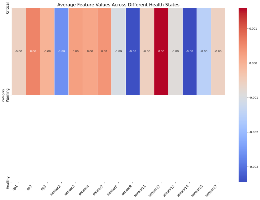
def analyze_failure_patterns(train_df, relevant_features, category_labels):
    """
    分析不同故障类别的特征模式

    参数:
    train_df: 训练数据
    relevant_features: 相关特征列表
    category_labels: 故障类别标签
    """
    # 首先检查长度兼容性
    print(f"训练数据长度: {len(train_df)}, 类别标签长度: {len(category_labels)}")

    # 创建副本以避免修改原始数据框
    analysis_df = train_df.copy()

    # 只使用与类别标签长度匹配的数据子集
    if len(analysis_df) != len(category_labels):
        print("警告: 长度不匹配。仅使用与类别标签长度匹配的数据前部分。")
        analysis_df = analysis_df.head(len(category_labels))

    # 将类别标签添加到数据框
    analysis_df['Category'] = category_labels

    # 计算每个类别的平均特征值
    category_means = analysis_df.groupby('Category')[relevant_features].mean()

    # 绘制热图
    plt.figure(figsize=(14, 10))
    sns.heatmap(category_means, annot=True, cmap='coolwarm', fmt='.2f', linewidths=.5)
    plt.title('不同健康状态下的平均特征值', fontsize=16)
    plt.xticks(rotation=45, ha='right', fontsize=12)
    plt.yticks([0, 1, 2], ['临界状态', '警告状态', '健康状态'], fontsize=12)
    plt.tight_layout()
    plt.show()

    # 绘制每个类别的特征分布
    for feature in relevant_features[:5]:  # 仅显示前5个特征以避免过多图表
        plt.figure(figsize=(12, 8))
        for category in range(3):
            cat_data = analysis_df[analysis_df['Category'] == category][feature]
            sns.kdeplot(cat_data, label=f'类别 {category}')

        plt.title(f'特征分布: {feature}', fontsize=16)
        plt.xlabel('标准化值', fontsize=14)
        plt.ylabel('密度', fontsize=14)
        plt.legend(['临界状态', '警告状态', '健康状态'])
        plt.grid(True, linestyle='--', alpha=0.7)
        plt.tight_layout()
        plt.show()

# 5. 主函数
def main():

    # 加载数据
    train_df, test_df, rul_df = load_data(train_file, test_file, rul_file)

    # 预处理数据
    train_df, relevant_features = preprocess_data(train_df, is_training=True)
    test_df, _ = preprocess_data(test_df, is_training=False)

    # 保存原始train_df以供后续使用
    original_train_df = train_df.copy()

    # 创建序列数据
    sequence_length = 30 
    X_train, y_train = create_sequences(train_df, sequence_length)

    # 构建自编码器模型
    input_shape = X_train.shape[1:]  # 序列长度 x 特征数量
    autoencoder, encoder = build_autoencoder(input_shape, encoding_dim=16)

    # 模型训练
    early_stopping = EarlyStopping(monitor='val_loss', patience=10, restore_best_weights=True)
    history = autoencoder.fit(
        X_train, X_train,
        epochs=100,
        batch_size=64,
        validation_split=0.2,
        callbacks=[early_stopping],
        verbose=1
    )

    # 提取编码特征
    encoded_features = encoder.predict(X_train)

    # 根据RUL值对样本进行分类
    category_labels = categorize_rul(y_train)

    # t-SNE可视化
    visualize_tsne(encoded_features, category_labels, 't-SNE编码特征可视化')

    # 计算重构误差
    reconstruction_errors = calculate_reconstruction_error(autoencoder, X_train)

    # 可视化重构误差与RUL的关系
    plt.figure(figsize=(12, 8))
    plt.scatter(y_train, reconstruction_errors, c=category_labels, cmap='viridis', alpha=0.6)
    plt.title('重构误差与剩余使用寿命(RUL)的关系', fontsize=16)
    plt.xlabel('剩余使用寿命(RUL)', fontsize=14)
    plt.ylabel('重构误差', fontsize=14)
    plt.colorbar(label='健康状态类别')
    plt.grid(True, linestyle='--', alpha=0.7)
    plt.tight_layout()
    plt.show()

    # 分析特征重要性
    # 首先需要提取特征名称（删除unit、cycle、RUL列）
    feature_names = train_df.drop(['unit', 'cycle', 'RUL'], axis=1).columns
    importance_df = analyze_feature_importance(encoder, feature_names)
    plot_feature_importance(importance_df)

    print("\n正在准备故障模式分析数据...")
    original_rul = original_train_df['RUL'].values
    original_categories = categorize_rul(original_rul)


    min_length = min(len(original_categories), len(category_labels))
    print(f"使用 {min_length} 个样本进行故障模式分析")

    # 现在使用匹配的长度进行分析
    analyze_failure_patterns(original_train_df.head(min_length), relevant_features, category_labels[:min_length])

    # 输出结果摘要
    print("分析完成！根据自编码器和t-SNE可视化结果，我们可以得出以下结论：")
    print("1. 涡扇发动机故障模式特征：")
    print("   - 从t-SNE可视化中可以观察到不同健康状态的聚类")
    print("   - 重构误差与RUL之间存在明显相关性")
    print("\n2. 最重要的故障指示特征：")
    for i, (feature, importance) in enumerate(zip(importance_df['Feature'].head(5),
                                                 importance_df['Importance'].head(5))):
        print(f"   {i+1}. {feature}: {importance:.4f}")

    print("\n3. 建议的维护措施：")
    print("   - 当重构误差超过阈值时应进行预防性维护")
    print("   - 对于存在异常传感器读数的发动机，应优先检查与上述关键传感器对应的组件")
    print("   - 根据RUL预测建立维护计划，在达到临界故障状态之前进行检查")

if __name__ == "__main__":
    main()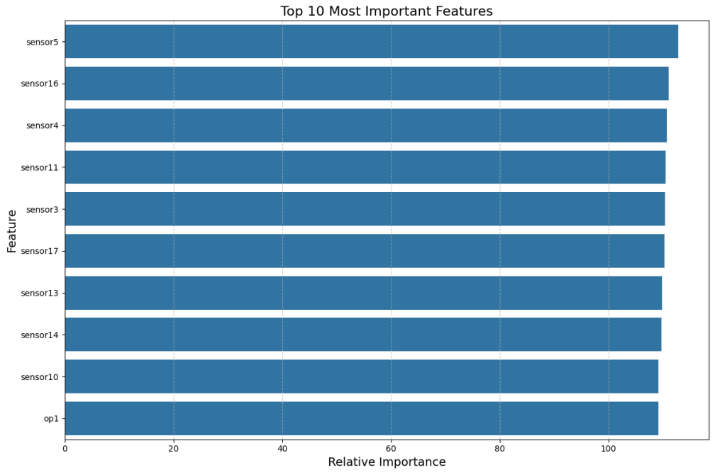

四、小结

设计一个完整的航空发动机健康监测与故障诊断系统，通过自编码器进行特征学习，实现了：

1. 健康状态分类：将发动机运行状态分为临界、警告和健康三类
2. 故障特征识别：识别出对故障预测最重要的传感器指标
3. 异常检测能力：通过重构误差检测异常运行状态
4. 维护决策支持：为预防性维护提供数据驱动的决策依据

该系统可以应用于航空发动机的预测性维护，通过及时发现潜在故障模式，有效减少非计划停机时间，提高安全性并降低维护成本。该方法也可扩展到其他工业设备的健康监测与故障诊断领域。