coursera机器学习课程笔记 第三周 逻辑回归

ex2

github:https://github.com/DLW3D/coursera-machine-learning-ex
练习文件下载地址:https://s3.amazonaws.com/spark-public/ml/exercises/on-demand/machine-learning-ex2.zip

Logistic Regression 逻辑回归

Sigmoid Function Sigmoid函数

sigmoid.m

function g = sigmoid(z)
	g=1 ./ (1 + exp(-z));
end

Cost Function 代价函数

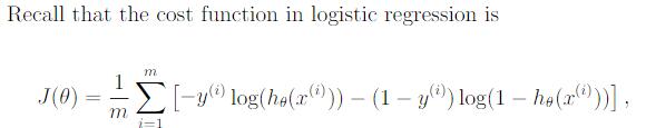
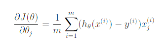
costFunction.m

function [J, grad] = costFunction(theta, X, y)
	m = length(y); 
	h = sigmoid(X*theta);%1*m
	J = sum(-y .* log(h) - (1-y).*log(1-h))/m;%1
	grad = ((h-y)'*X/m)';%n*1
end

Predict 预测函数

predict.m

function p = predict(theta, X)
	m = size(X, 1); % Number of training examples
	lambda=0.5;
	r = sigmoid(X * theta);%m*1
	p = floor(r+lambda);
end

Regularized Logistic Regression 正则化逻辑回归代价函数

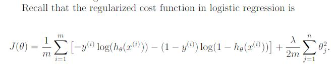
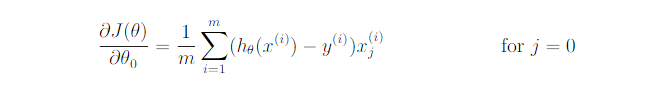
costFunctionReg.m

function [J, grad] = costFunctionReg(theta, X, y, lambda)
	m = length(y); % number of training examples
	n = size(theta);
	h = sigmoid(X*theta));%1*m
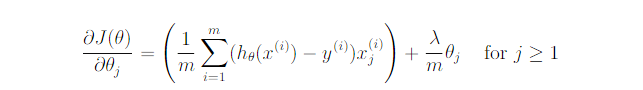
	J = sum(-y .* log(h) - (1-y).*log(1-h))/m + lambda/2/m.*theta(2:n)'*theta(2:n);%1
	grad1 = ((h-y)'*X(:,1)/m)';%1*1
	grad2 = ((h-y)'*X(:,2:n)/m)'+lambda/m.*theta(2:n);%n*1
	grad = [grad1;grad2];
end

运行逻辑回归

data = load('ex2data1.txt');
X = data(:, [1, 2]); y = data(:, 3);

%  Setup the data matrix appropriately, and add ones for the intercept term
[m, n] = size(X);

% Add intercept term to x and X_test
X = [ones(m, 1) X];

% Initialize fitting parameters
initial_theta = zeros(n + 1, 1);

%  Set options for fminunc
options = optimset('GradObj', 'on', 'MaxIter', 400);

%  Run fminunc to obtain the optimal theta
%  This function will return theta and the cost 
[theta, cost] = fminunc(@(t)(costFunction(t, X, y)), initial_theta, options);

% Plot Boundary
plotDecisionBoundary(theta, X, y);

% Put some labels 
hold on;
% Labels and Legend
xlabel('Exam 1 score')
ylabel('Exam 2 score')

% Specified in plot order
legend('Admitted', 'Not admitted')
hold off;

运行正规化逻辑回归

data = load('ex2data2.txt');
X = data(:, [1, 2]); y = data(:, 3);
X = mapFeature(X(:,1), X(:,2));

% Initialize fitting parameters
initial_theta = zeros(size(X, 2), 1);

% Set regularization parameter lambda to 1 (you should vary this)
for lambda = [0,1,10,100]

% Set Options
options = optimset('GradObj', 'on', 'MaxIter', 400);

% Optimize
[theta, J, exit_flag] = ...
	fminunc(@(t)(costFunctionReg(t, X, y, lambda)), initial_theta, options);

% Plot Boundary
plotDecisionBoundary(theta, X, y);
hold on;
title(sprintf('lambda = %g', lambda))

% Labels and Legend
xlabel('Microchip Test 1')
ylabel('Microchip Test 2')

legend('y = 1', 'y = 0', 'Decision boundary')
hold off;

% Compute accuracy on our training set
p = predict(theta, X);

fprintf('Train Accuracy: %f\n', mean(double(p == y)) * 100);
fprintf('Expected accuracy (with lambda = 1): 83.1 (approx)\n');
end

mapFeature.m

function out = mapFeature(X1, X2)
% MAPFEATURE Feature mapping function to polynomial features
%
%   MAPFEATURE(X1, X2) maps the two input features
%   to quadratic features used in the regularization exercise.
%
%   Returns a new feature array with more features, comprising of 
%   X1, X2, X1.^2, X2.^2, X1*X2, X1*X2.^2, etc..
%
%   Inputs X1, X2 must be the same size
%

degree = 6;
out = ones(size(X1(:,1)));
for i = 1:degree
    for j = 0:i
        out(:, end+1) = (X1.^(i-j)).*(X2.^j);
    end
end

end