


接触过深度学习的朋友对MNIST数据集肯定不陌生。基本上算是玩神经网络里的“hello,world!”
本节基于MNIST数据集,实现CNN学习过程。
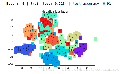
下面是一个 CNN 最后一层的学习过程, 我们先可视化看看:

MNIST手写数据
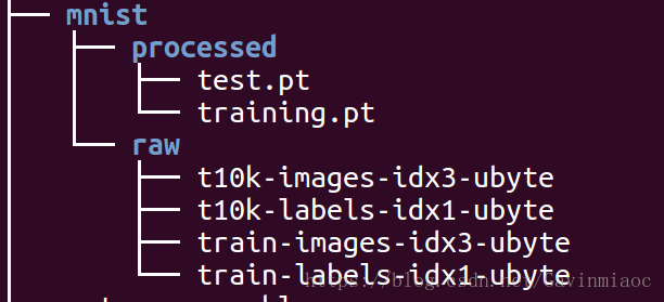
首先是数据集下载,为了看看数据集里究竟是长什么样子的,我也作了展示:
# library
# standard library
import os

# third-party library
import torch
import torch.nn as nn
from torch.autograd import Variable
import torch.utils.data as Data
import torchvision
import matplotlib.pyplot as plt

torch.manual_seed(1)    # reproducible

# Hyper Parameters
EPOCH = 1               # train the training data n times, to save time, we just train 1 epoch
BATCH_SIZE = 50
LR = 0.001              # learning rate
DOWNLOAD_MNIST = False


# Mnist digits dataset
if not(os.path.exists('./mnist/')) or not os.listdir('./mnist/'):
    # not mnist dir or mnist is empyt dir
    DOWNLOAD_MNIST = True

train_data = torchvision.datasets.MNIST(
    root='./mnist/',
    train=True,                                     # this is training data
    transform=torchvision.transforms.ToTensor(),    # Converts a PIL.Image or numpy.ndarray to
                                                    # torch.FloatTensor of shape (C x H x W) and normalize in the range [0.0, 1.0]
    download=DOWNLOAD_MNIST,
)

# plot one example
print(train_data.train_data.size())                 # (60000, 28, 28)
print(train_data.train_labels.size())               # (60000)
plt.imshow(train_data.train_data[0].numpy(), cmap='gray')
plt.title('%i' % train_data.train_labels[0])
plt.show()
结果如下:
首先看下载后的数据集目录
展示example
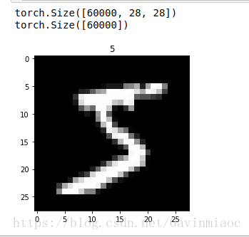
黑色的地方的值都是0, 白色的地方值大于0.
同样, 我们除了训练数据, 还给一些测试数据, 测试看看它有没有训练好
CNN模型 
和以前一样, 我们用一个 class 来建立 CNN 模型. 这个 CNN 整体流程是 卷积(Conv2d) -> 激励函数(ReLU) -> 池化, 向下采样 (MaxPooling) -> 再来一遍 -> 展平多维的卷积成的特征图 -> 接入全连接层 (Linear) -> 输出
# Data Loader for easy mini-batch return in training, the image batch shape will be (50, 1, 28, 28)
train_loader = Data.DataLoader(dataset=train_data, batch_size=BATCH_SIZE, shuffle=True)

# convert test data into Variable, pick 2000 samples to speed up testing
# # 为了节约时间, 我们测试时只测试前2000个
test_data = torchvision.datasets.MNIST(root='./mnist/', train=False)
test_x = Variable(torch.unsqueeze(test_data.test_data, dim=1), volatile=True).type(torch.FloatTensor)[:2000]/255.   # shape from (2000, 28, 28) to (2000, 1, 28, 28), value in range(0,1)
test_y = test_data.test_labels[:2000]


class CNN(nn.Module):
    def __init__(self):
        super(CNN, self).__init__()
        self.conv1 = nn.Sequential(         # input shape (1, 28, 28)
            nn.Conv2d(
                in_channels=1,              # input height
                out_channels=16,            # n_filters
                kernel_size=5,              # filter size
                stride=1,                   # filter movement/step
                padding=2,                  # if want same width and length of this image after con2d, padding=(kernel_size-1)/2 if stride=1
            ),                              # output shape (16, 28, 28)
            nn.ReLU(),                      # activation
            nn.MaxPool2d(kernel_size=2),    # choose max value in 2x2 area, output shape (16, 14, 14)
        )
        self.conv2 = nn.Sequential(         # input shape (16, 14, 14)
            nn.Conv2d(16, 32, 5, 1, 2),     # output shape (32, 14, 14)
            nn.ReLU(),                      # activation
            nn.MaxPool2d(2),                # output shape (32, 7, 7)
        )
        self.out = nn.Linear(32 * 7 * 7, 10)   # fully connected layer, output 10 classes

    def forward(self, x):
        x = self.conv1(x)
        x = self.conv2(x)
        x = x.view(x.size(0), -1)           # flatten the output of conv2 to (batch_size, 32 * 7 * 7)
        output = self.out(x)
        return output, x    # return x for visualization


cnn = CNN()
print(cnn)  # net architecture
结构打印如下:

训练
下面我们开始训练, 将 x y 都用 Variable 包起来, 然后放入 cnn 中计算 output, 最后再计算误差.
optimizer = torch.optim.Adam(cnn.parameters(), lr=LR) # optimize all cnn parameters
loss_func = nn.CrossEntropyLoss() # the target label is not one-hotted
# following function (plot_with_labels) is for visualization, can be ignored if not interested
from matplotlib import cm
try: from sklearn.manifold import TSNE; HAS_SK = True
except: HAS_SK = False; print('Please install sklearn for layer visualization')
def plot_with_labels(lowDWeights, labels):
plt.cla()
X, Y = lowDWeights[:, 0], lowDWeights[:, 1]
for x, y, s in zip(X, Y, labels):
c = cm.rainbow(int(255 * s / 9)); plt.text(x, y, s, backgroundcolor=c, fontsize=9)
plt.xlim(X.min(), X.max()); plt.ylim(Y.min(), Y.max()); plt.title('Visualize last layer'); plt.show(); plt.pause(0.01)
plt.ion()
# training and testing
for epoch in range(EPOCH):
for step, (x, y) in enumerate(train_loader): # gives batch data, normalize x when iterate train_loader
b_x = Variable(x) # batch x
b_y = Variable(y) # batch y
output = cnn(b_x)[0] # cnn output
loss = loss_func(output, b_y) # cross entropy loss
optimizer.zero_grad() # clear gradients for this training step
loss.backward() # backpropagation, compute gradients
optimizer.step() # apply gradients
if step % 50 == 0:
test_output, last_layer = cnn(test_x)
pred_y = torch.max(test_output, 1)[1].data.squeeze()
accuracy = sum(pred_y == test_y) / float(test_y.size(0))
print('Epoch: ', epoch, '| train loss: %.4f' % loss.data[0], '| test accuracy: %.2f' % accuracy)
if HAS_SK:
# Visualization of trained flatten layer (T-SNE)
tsne = TSNE(perplexity=30, n_components=2, init='pca', n_iter=5000)
plot_only = 500
low_dim_embs = tsne.fit_transform(last_layer.data.numpy()[:plot_only, :])
labels = test_y.numpy()[:plot_only]
plot_with_labels(low_dim_embs, labels)
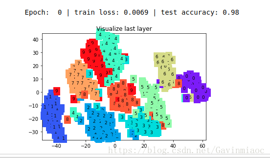
plt.ioff()训练过程展示:

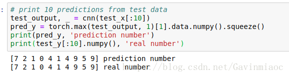
最后我们再来取10个数据, 看看预测的值到底对不对:
预测结果
可视化训练
因为可视化可以帮助理解, 所以还是有必要提一下. 可视化的代码主要是用 matplotlib 和 sklearn 来完成的, 因为其中我们用到了 T-SNE 的降维手段, 将高维的 CNN 最后一层输出结果可视化, 也就是 CNN forward 代码中的 x = x.view(x.size(0), -1) 这一个结果.


 243
243

 被折叠的 条评论
为什么被折叠?
被折叠的 条评论
为什么被折叠?
 到【灌水乐园】发言


