相关系数今世前生

相关系数今世前生

1. Introduction The complete name of the correlation coefficient deceives many students into a belief that Karl Pearson developed this statistical measure himself. Although Pearson did develop a rigorous treatment of the mathematics of the Pearson Product Moment Correlation (PPMC), it was the imagination of Sir Francis Galton that originally conceived modern notions of correlation and regression. Galton, a cousin of Charles Darwin and an accomplished 19th century scientist in his own right, has often been criticized in this century for his promotion of "eugenics" (planned breeding of humans; see, for example, Paul (1995). Historians have also suggested that his cousin's lasting fame unfairly overshadowed the substantial scientific contributions Galton made to biology, psychology and applied statistics (see, for example, FitzPatrick 1960). Galton's fascination with genetics and heredity provided the initial inspiration that led to regression and the PPMC. 中文(简体)
2. 介绍 相关系数的完整名称欺骗了许多学生，认为卡尔·皮尔森（Karl Pearson）自己开发了这个统计方法。尽管皮尔逊确实对皮尔逊产品矩相关（PPMC）的数学进行了严格的处理，但是弗朗西斯·高尔顿爵士的想象力最初构想了现代关联和回归的概念。查尔斯·达尔文（Charles Darwin）的堂弟和一位十九世纪成就卓着的科学家高尔顿（Galton）在本世纪因其促进“优生学”（有计划地繁殖人类;例如参见Paul（1995）也暗示了他的表兄长久的名望不公平地掩盖了高尔顿对生物学，心理学和应用统计学所作的实质性科学贡献（例如参见FitzPatrick，1960），Galton对遗传学和遗传的迷恋提供了导致衰退和PPMC的最初启发。

The thoughts that prompted the development of the PPMC began with a then vexing problem of heredity -- understanding how strongly the characteristics of one generation of living things manifested in the following generation. Galton initially approached this problem by examining characteristics of the sweet pea plant. He chose the sweet pea because that species could self-fertilize; daughter plants express genetic variations from mother plants without contribution from a second parent. This characteristic eliminated, or at least postponed, having to deal with the problem of statistically assessing genetic contributions from multiple sources. Galton's first insights about regression sprang from a two-dimensional diagram plotting the sizes of daughter peas against the sizes of mother peas. As described below, Galton used this representation of his data to illustrate basic foundations of what statisticians still call regression. The generalization of these efforts into the product-moment correlation and the more complex multiple regression came much later. Current textbooks of behavioral science statistics typically reverse this order: the PPMC is presented first and linear regression is covered later. Many instructors may also feel more comfortable starting with correlation and building up to regression. 中文(简体) 促使PPMC发展的思想始于一个令人头痛的遗传问题 - 理解一代代生物的特征在后代中的表现如何强烈。高尔顿最初通过研究甜豌豆植物的特征来解决这个问题。他选择了甜豌豆，因为这种物种可以自我施肥;子代植物表达来自母本植物的遗传变异而没有来自第二亲本的贡献。这个特点消除了，或者至少推迟了，不得不处理统计评估来自多个来源的遗传贡献的问题。高尔顿关于回归的第一次见解是从绘制豌豆大小和母豌豆大小的二维图表中跳出来的。如下所述，高尔顿用这些数据表示他的数据来说明什么统计学家仍称为回归的基础。将这些努力推广到产品时刻相关性和更复杂的多元回归中的时间要晚得多。行为科学统计学的现行教科书通常会颠倒这个顺序：首先介绍PPMC，稍后介绍线性回归。许多教师也可能从相关性和回归开始感觉更舒适。 The present paper provides historical background and illustrative examples that statistics instructors may find useful in introducing these concepts to college level classes in applied statistics. By briefly tracing the historical development of regression and correlation, this paper shows how introductory statistics instructors can use engaging and historically accurate examples to introduce regression and correlation to students. A number of articles concerning the teaching of regression and correlation indicate that students often have difficulty understanding these concepts and the connection between them (see, for example, Williams 1975; Duke 1978; Karylowski 1985; Goldstein and Strube 1995;). The present article provides new ideas for instruction based on the historical origins of these statistical techniques. 中文(简体) 本文提供了历史背景和说明性的例子，统计指导者可能会发现在应用统计学中将这些概念引入到大学水平课程中是有用的。通过简要回顾回归和相关的历史发展，本文展示了引导统计教师如何使用引人入胜和历史准确的例子来向学生介绍回归和相关性。一些关于回归和相关性教学的文章指出，学生往往难以理解这些概念及其之间的联系（例如，Williams 1975; Duke 1978; Karylowski 1985; Goldstein and Strube 1995）。本文根据这些统计技术的历史渊源提供了新的教学思想。

2.高尔顿对回归的早期考虑

• Besides his role as a colleague of Galton's and a researcher in Galton's laboratory, Karl Pearson also became Galton's biographer after the latter's death in 1911 (Pearson 1922). In his four-volume biography of Galton, Pearson described the genesis of the discovery of the regression slope (Pearson 1930). In 1875, Galton had distributed packets of sweet pea seeds to seven friends; each friend received seeds of uniform weight (also see Galton 1894), but there was substantial variation across different packets. Galton's friends harvested seeds from the new generations of plants and returned them to him (see Appendix A). Galton plotted the weights of the daughter seeds against the weights of the mother seeds. Galton realized that the median weights of daughter seeds from a particular size of mother seed approximately described a straight line with positive slope less than 1.0:

• 中文(简体)

• 除了他作为高尔顿的同事和高尔顿实验室的研究人员以外，卡尔·皮尔逊（Karl Pearson）在1911年死后也成为高尔顿的传记作者（皮尔逊1922年）。皮尔逊在他的四卷高尔顿传记中描述了发现回归斜坡的起源（Pearson，1930）。 1875年，高尔顿向七位朋友分发了甜豌豆种子。每个朋友收到统一重量的种子（也见Galton 1894），但是不同的数据包有很大的差异。高尔顿的朋友们收获了新一代植物的种子，并将其归还给他（参见附录A）。加尔顿绘制了女儿种子的重量与母亲种子的重量之间的关系。高尔顿意识到，从一个特定的母亲种子大小的女儿种子的中等重量近似描述了一个正斜率小于1.0的直线：

• Thus he naturally reached a straight regression line, and the constant variability for all arrays of one character for a given character of a second. It was, perhaps, best for the progress of the correlational calculus that this simple special case should be promulgated first; it is so easily grasped by the beginner.

• 中文(简体)

• 因此，他自然而然地达到了一条直线回归线，并且一个字符的所有阵列对于给定的一秒字符的恒定可变性。也许，对于相关演算的进展来说，这个简单的特例最好先发布一下。这是初学者很容易掌握的。

• The simple, special case that Pearson referred to is, of course, both the roughly equivalent variability of the two measures and their identical units of measurement. Figure 1 uses a simple, invented data set to illustrate Galton's earliest findings. The parent sweet pea size on the X-axis and the offspring sweet pea size on the Y-axis have approximately equal variability. Thus, the slope of the line connecting the means of the different columns of points is equivalent both to the regression slope and the correlation coefficient. For Galton's purposes, any slope smaller than 1.0 indicated regression to the mean for that generation of peas. The phenomenon of regression to the mean is illustrated by the configuration of points: The y-coordinates of most of the points in Figure 1 are closer to the horizontal offspring mean than their x-coordinates are to the vertical parent mean. Galton's first documented study of this type suggested a slope of 0.33 (obtained through careful inspection of his scatterplots), which indicated to him that extremely large or small mother seeds typically generated substantially less extreme daughter seeds. This finding is, of course, prototypical of regression to the mean: For many variables, natural processes work to "dampen" extreme outliers and bring them closer to their respective means.

• 中文(简体)

• Pearson提到的简单而特殊的情况当然是两个度量的大致相等的变化以及它们相同的度量单位。图1使用一个简单的，发明的数据集来说明高尔顿最早的发现。 X轴上的亲本甜豌豆大小和Y轴上的后代甜豌豆大小具有大致相等的变异性。因此，连接不同列点的平均线的斜率等于回归斜率和相关系数。对于高尔顿的目的，任何小于1.0的斜率都表示回归到那一代豌豆的平均值。回归到均值的现象由点的构型来说明：图1中大多数点的y坐标比它们的x坐标更接近水平后代平均值，而垂直父平均值更接近水平后代平均值。高尔顿第一次记录的这种类型的研究表明0.33的坡度（通过仔细检查他的散点图获得），这表明极大或小的母本通常产生极少的极端女儿的种子。这个发现当然是回归平均值的原型：对于许多变量，自然过程的作用是“抑制”极端的异常值，并使它们更接近它们各自的手段。

• Figure 1. Connecting the means of the individual columns of data provides a crude approximation of the regression line. The slope is exactly 0.50 and the correlation is approximately r = 0.51. Many, though not all, of the points are closer to the offspring pea size mean of 9 on the Y-axis than to the parental pea size mean of 10 on the X-axis. The numeric data appear in Appendix B.

• 中文(简体)

• 图1.连接各个数据列的方法提供了回归线的粗略近似。斜率恰好为0.50，相关性约为r = 0.51。许多（但不是全部）的点在Y轴上比后代豌豆大小平均值9更接近X轴上的亲本豌豆大小平均值10。数值数据见附录B.

• Nonetheless, only a horizontal line would have indicated no heritability in seed size whatsoever, so Galton's finding affirmed his basic assumptions concerning the heritability of "characters." Figure 1, greatly simplified from Galton's original graph, illustrates how a line connecting the means of the columns of data points indicates the degree to which extreme values in the first generation (on the X-axis) tend to regress toward the mean of the second generation (on the Y-axis). I invented the data points, which are listed in Appendix B, to simplify hand calculation in a classroom setting. In contrast to Figure 1, Galton's original data did not produce a perfectly smooth line, but he was able to draw, by hand, a single line that fit all the data reasonably well (Galton's first regression line was presented at a lecture in 1877; see (Pearson 1930). The slope of this line he designated "r" for regression. Only under Pearson's later treatment did r come to stand for the correlation coefficient (Pearson 1896).

• 中文(简体)

• 尽管如此，只有一条水平线才会表明种子大小没有遗传力，所以高尔顿的发现肯定了他对“人物”遗传性的基本假设。图1从Galton的原始图中大大简化，说明连接数据点列的方法的线如何表示第一代（在X轴上）的极值趋向于向第二个代（在Y轴上）。我发明了附录B中列出的数据点，以简化课堂环境下的手工计算。与图1相比，高尔顿的原始数据并没有产生一个完美的平滑线，但是他能够用一个单一的线来合理地拟合所有的数据（高尔顿的第一条回归线是在1877年的演讲中提出的; （Pearson，1930），这条线的斜率用“r”表示，只有在Pearson的后期处理中，r才能代表相关系数（Pearson，1896）。

• Galton's progress was both eased and hobbled by his choices for descriptive statistics; he used the median as a measure of central tendency and the semi-interquartile range as a measure of variability. One advantage of these measures lay in the simplicity of obtaining them. Galton was nearly fanatical about graphing and tabulating every available data point. These descriptive values could emerge from an inspection of the resulting figure or table with a minimum of computation. It is understood now that the median and semi-interquartile range do not have the favorable mathematical properties of the mean and standard deviation (for example, they cannot be manipulated using covariance algebra). But Galton was not a sophisticated enough mathematician to recognize the deficiency. So Galton's progress toward a more general implementation of regression was delayed by his choice of descriptive statistics. In Natural Inheritance (Galton 1894), Galton expended a page or two making various arguments about the exact value of the slope of a regression line as calculated with various techniques to estimate the change in Y versus the change in X on the scatterplot. At that point in time, his efforts lacked the mathematical foundation to derive the slope from the data themselves. As an interesting footnote, in the late 1870s, Galton did not have access to a mechanical calculating machine, whereas Pearson had one for personal use on his desk no later than 1910 (Pearson 1938).

• 中文(简体)

• 高尔顿的进步既得到了描述性统计的选择，也得到了缓解，他用中位数作为衡量中心趋势的指标，用半四分位间距作为衡量变异性的指标。这些措施的一个优点在于获得它们的简单性。高尔顿几乎是狂热的绘制和列表每个可用的数据点。这些描述性的价值可以通过以最少的计算检查所得到的图形或表格而出现。现在可以理解，中位数和半四分位数范围不具有均值和标准差的有利数学性质（例如，不能用协方差代数来操纵）。但高尔顿并不是一个足够复杂的数学家来认识这个缺陷。因此，高尔顿在更普遍的回归方面取得的进展，被他选择的描述性统计推迟了。在“自然遗产”（Galton 1894）中，高尔顿花费了一两页时间，用各种技术计算回归线的斜率的确切值，以估计Y与散点图上X的变化。在那个时候，他的努力缺乏从数据本身得出斜率的数学基础。作为一个有趣的脚注，在十九世纪七十年代后期，高尔顿没有机械计算机，而皮尔森最晚在1910年在皮尔逊的桌子上有个人使用（皮尔逊1938年）。

• 3.高尔顿对回归斜率普遍性的认识

• Even with his poor choice of descriptive statistics, Galton was able to generalize his work over a variety of heredity problems. He tackled personality temperament, artistic ability, and disease incidence, among others (Galton 1894). The important breakthrough in the process of analyzing these data came from his realization that if the degree of association between two variables was held constant, then the slope of the regression line could be described if the variability of the two measures were known. At that time Galton believed he had estimated a single heredity constant that was generalizable to many or most inherited characteristics. But he wondered why, if such a constant existed, the observed slopes in his parent-child plots varied so much over these characteristics. After noticing differences in variability between generations, he arrived at the idea that the differences in regression slopes that he obtained were solely due to differences in variability between the different sets of measurements. 即使他描述性统计数据的选择不佳，高尔顿也能够将他的工作概括为各种遗传问题。他解决了性格气质，艺术能力和疾病发生等（Galton 1894）。分析这些数据过程中的重要突破来自他认识到，如果两个变量之间的关联程度保持不变，则可以描述回归线的斜率，如果两个度量的变化性已知。当时，高尔顿相信他估计了一种单一的遗传常数，这种遗传常数可以归纳为许多或最具遗传特征。但他想知道为什么如果存在这样一个常数，他的父母 - 子女情节中观察到的斜坡在这些特征上差异很大。在注意到世代之间差异的差异之后，他得出这样的观点：他获得的回归斜率的差异仅仅是由于不同组测量之间变化的差异。

• In modern terms, this principle can be illustrated by assuming a constant correlation coefficient but varying the standard deviations of the two variables involved. Figures 2A, B, and C display the scatterplots of three closely related data sets. The correlation in each data set is identical at r = 0.64 (note that 0.66 was one of the basic heritability constants derived by Galton). In Figure 2A the standard deviation of Y is the same as the standard deviation of X. In Figure 2B the standard deviation of Y is smaller than the standard deviation of X. Finally, in Figure 2C the standard deviation of Y is larger than the standard deviation of X. The data, which appear in Appendix B, were designed to center both variables on zero and to simplify hand calculations for classroom use. The scales of measurement are arbitrary. Anchoring a straight edge or ruler at the origin, one can estimate the slope of the line of best fit: the line becomes shallower as the variability of Y decreases relative to the variability of X and steeper as variability of Y increases relative to the variability of X. 用现代术语来说，这个原则可以通过假定一个恒定的相关系数来说明，但是可以改变所涉及的两个变量的标准偏差。图2A，B和C显示三个紧密相关的数据集的散点图。每个数据集中的相关性在r = 0.64时是相同的（注意，0.66是由Galton得出的基本遗传力常数之一）。在图2A中，Y的标准偏差与X的标准偏差相同。在图2B中，Y的标准偏差小于X的标准偏差。最后，在图2C中，Y的标准偏差大于标准偏差X的偏差。出现在附录B中的数据旨在将两个变量置于零中，并简化课堂使用的手动计算。度量的尺度是任意的。在原点处固定一条直边或标尺，可以估计最佳拟合线的斜率：随着Y的变化相对于X的变化而减小并且随着Y的变化相对于变化X X。

• Figure 2. Correlation remains constant even though the slope of the line changes as a result of differences in variability between the two variables. In all three graphs, the correlation is identical at approximately r = 0.64. In 2A the variability in X is identical to the variability in Y. In 2B the variability in X was magnified to be larger than the variability in Y. In 2C the variability in Y was magnified to be larger than the variability in X. The numeric data appear in Appendix B. 图2.即使线的斜率由于两个变量之间的变化差异而变化，相关性仍然保持不变。 在所有三个图中，相关性在大约r = 0.64处是相同的。 在2A中，X中的变异性与Y中的变异性相同。在2B中，X中的变异性被放大为大于Y中的变异性。在2C中，Y中的变异性被放大为大于X中的变异性。数字 数据出现在附录B中。

• Although he represented it with different symbols, Galton had at this point recognized that the rudimentary regression equation y = r ( Sy / Sx ) x described the relationship between his paired variables. Galton used an estimated value of r, because he did not know how to calculate it. The expression (Sy / Sx) was, in effect, a correction factor that allowed him to adjust the observed slope based on the variability of each measure. Modern work on genetics and inheritance has not supported Galton's belief in a universal heritability constant (that is, a fixed correlation of characteristics across generations), but this mistaken assumption gave him the impetus to advance the conceptual division between correlation and regression. As represented in Figure 2, the visible squashing and stretching of the X and Y distributions across the three figures does not hide the evident relationship between the two variables. The degree of association between the two variables remains constant even though the slope of the line is different in all three graphs. Galton correctly recognized that the ratio of variabilities of the two measures was a key factor in determining the slope of the regression line. 虽然他用不同的符号表示，但高尔顿在这一点上认识到，最初的回归方程y = r（Sy / Sx）x描述了他的配对变量之间的关系。高尔顿使用r的估计值，因为他不知道如何计算它。表达式（Sy / Sx）实际上是一个校正因子，允许他根据每个度量的可变性来调整观察到的斜率。关于遗传学和遗传学的现代研究并没有支持高尔顿对普遍遗传力常数的信念（即跨越世代的特征的固定相关性），但是这个错误的假设促使他推动了相关和回归之间的概念划分。如图2所示，三个图中X和Y分布的可见挤压和拉伸并不掩盖两个变量之间的明显关系。即使在所有三个图中线的斜率不同，两个变量之间的关联程度仍然保持不变。高尔顿正确地认识到两个度量的变化率是决定回归线斜率的关键因素。

4.皮尔逊关联与回归的数学发展

In 1896, Pearson published his first rigorous treatment of correlation and regression in the Philosophical Transactions of the Royal Society of London . In this paper, Pearson credited Bravais (1846) with ascertaining the initial mathematical formulae for correlation. Pearson noted that Bravais happened upon the product-moment (that is, the "moment" or mean of a set of products) method for calculating the correlation coefficient but failed to prove that this provided the best fit to the data. Using an advanced statistical proof (involving a Taylor expansion), Pearson demonstrated that optimum values of both the regression slope and the correlation coefficient could be calculated from the product-moment, \frac{\sum xy}{n}, where x and y are deviations of observed values from their respective means and n is the number of pairs. For example, in linear regression, if the slope is calculated from the product-moment, then the observed x values predict the observed y values with the minimum possible sum of squared errors of prediction, \sum{Y-Y-hat}^2.

1896年，皮尔逊在伦敦皇家学会的哲学交易中发表了他的第一个严谨的关联和回归处理。在本文中，皮尔逊将布拉维斯（1846年）记为确定相关性的初始数学公式。 Pearson指出，布拉维发生在计算相关系数的产品时刻（即“时刻”或一组产品的平均值）方法，但未能证明这提供了最适合数据的方法。 Pearson利用一种先进的统计证据（涉及泰勒展开）证明了回归斜率和相关系数的最优值可以通过乘积矩来计算，其中x和y观测值与它们各自的平均值有偏差，n是成对的数量。例如，在线性回归中，如果从产品时刻计算斜率，则观察到的x值用预测的平方误差的最小可能总和来预测观察到的y值，其中y = Y_y-hat} ^ 2。

A simpler proof than Pearson's for the product-moment method appeared in Ghiselli (1981). Although neither Pearson's nor Ghiselli's proof is likely to enhance the flow of a typical introductory statistics class, a simple numerical re-creation of Ghiselli's proof can illuminate the important point about the optimal prediction of y from x. Such an example appears in Table 1. This table uses pairs of deviation scores to help demonstrate that the expression y-hat= b x minimizes squared prediction errors when b is calculated as the product-moment. The first three columns demonstrate the calculation of b as the mean (moment) of the products of the deviation scores. Both x and y vectors are centered on 0 so that each score is itself a deviation score. The rightmost four columns of Table 1 show that adding a small offset to the value of b or subtracting a small offset from b enlarges the sum of the squared errors of prediction. Both Ghiselli's and Pearson's proofs demonstrate more generally that any departure from the product-moment worsens the prediction of y from x.

Ghiselli（1981）提出了一个比Pearson的产品时刻方法更简单的证明。虽然皮尔逊和Ghiselli的证明都不可能增强典型的入门统计学课程的流程，但Ghiselli的证明的简单数值重新创造可以阐明关于y的最优预测的重要观点。表1显示了这样一个例子。这个表格使用偏差分数对来帮助证明当b被计算为产品时刻时，表达式y-hat = b x使平方预测误差最小化。前三列显示计算b作为偏差分数乘积的平均值（矩）。 x和y向量都以0为中心，这样每个分数本身就是一个偏差分数。表1最右边的四列表明，给b的值加上一个小的偏移量，或者从b中减去一个小的偏移量，就可以扩大预测误差的平方和。 Ghiselli's和Pearson的证明都更一般地表明，从产品时刻的任何偏离都会恶化对x的预测。

5.关于多元回归的注释

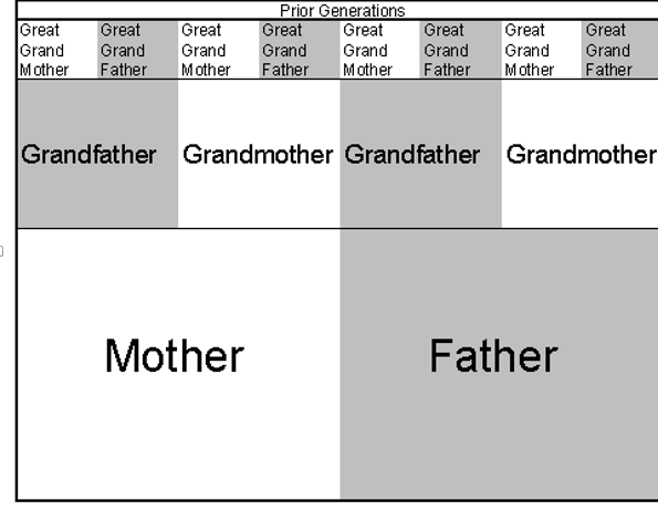
Galton realized soon after he had collected and analyzed his sweet pea data that the generations prior to the immediate parents could also influence individual characteristics (Pearson 1930). He even noticed that certain characteristics occasionally skipped one or more generations; a man may appear more similar to his grandfather than to his father in certain respects. In an 1898 paper to the journal Nature (cited in Pearson 1930), Galton published a clever diagram that partitioned a unit square into successively smaller squares, where each square represented the ever diminishing influence of previous generations of ancestors on the present individual. A modified and simplified version of the diagram appears in Figure 3. Within each row, smaller and smaller divisions represented each ancestor. Traveling backward through time, each generation had only half as much influence on the present individual as the generation succeeding it. 高尔顿在收集并分析他的甜豌豆数据之后不久就意识到，直系父母之前的世代也可能影响个人特征（Pearson 1930）。 他甚至注意到某些特征偶尔会跳过一代或更多代; 在某些方面，一个男人看起来更像他的祖父，而不是他的父亲。 在1898年发表于“自然”杂志（皮尔逊1930年引用）的一篇论文中，高尔顿发表了一个巧妙的图表，将单位正方形分割成更小的正方形，每个正方形表示前几代祖先对当前个体的影响力不断下降。 该图的修改和简化版本如图3所示。在每一行中，越小越小代表每个祖先。 随着时间的推移，每一代人对当代人的影响力只有一代人的一半。

Figure 3. Simplified diagram showing influences of three preceding generations of ancestors on the present day individual. 图3.显示前三代祖先对当代个体的影响的简图。

With the realization of this diminishing effect, Galton had hit upon the kernel of the idea of multiple regression. A characteristic or variable may be influenced not simply by a single important cause but by a multitude of causes of greater and lesser importance. Some of these causes may even overlap with one another (that is, the predictors themselves are intercorrelated). In later publications Galton listed some mathematical formulae that captured this same basic idea, but he was never able to develop a complete mathematical treatment of the matter:

"The somewhat complicated mathematics of multiple correlation, with its repeated appeals to the geometrical notions of hyperspace, remained a closed chamber to him." (Pearson 1930, p. 21) 随着这种递减效应的实现，高尔顿已经触及了多元回归思想的核心。 一个特征或变量可能不仅仅受到单一重要原因的影响，而且受到影响程度越来越大的多种原因的影响。 其中一些原因甚至可能与另一个原因重叠（即预测变量本身互相关联）。 在后来的出版物中，高尔顿列出了一些数学公式，这些公式包含了相同的基本思想，但是他从未能够对这个问题进行完整的数学处理：

“多重相关的有些复杂的数学，反复呼吁超空间的几何概念，对他来说仍然是一个封闭的房间。” （皮尔逊1930年，第21页）

Nonetheless, Galton's conceptualization of the multiple influences of progenitors on characteristics of the present day individual was entirely parallel to the modern conception of multiple regression. As with simple linear regression and the correlation coefficient, Galton laid the imaginative groundwork that Pearson later developed into a rigorous mathematical treatment. Pearson's subsequent work included further development of multiple regression as well as innovative progress on other statistics such as chi-square (Pearson 1938). 尽管如此，高尔顿关于祖先对当代个体特征的多重影响的概念化与现代多元回归概念完全平行。 与简单的线性回归和相关系数一样，高尔顿奠定了皮尔森后来发展成为严谨的数学治疗的想象基础。 培生的后续工作包括多元回归的进一步发展以及卡方等其他统计方面的创新进展（Pearson，1938）。

6.教学理念

The previous discussion of the development of regression and the correlation coefficient provides a historical account of aspects of scientific and mathematical progress in the late 1800s and early 1900s. In conjunction with the graphical and numerical examples presented, classroom use of some of these historical examples may improve comprehension and sustain student interest by showing the various problems that Galton, Pearson, and others struggled with and solved as they worked out the techniques that are so widely used today. The historical account describes a series of small conceptual steps that an instructor could package into one or more lectures for an introductory statistics class.

Such a series might begin with a brief overview of the heredity problems that Galton was considering. The simulated sweet pea data from Figure 1 illustrate the basic concepts of plotting data in columns, regression to the mean, and hand fitting a line to the data using the means of the columns. Galton's actual sweet pea data are summarized in Appendix A, and readers may request a copy of the complete data set from the author. The complete data set could be analyzed and plotted for classroom use with any statistical program. The instructor might also wish to plot an additional example of total regression to the mean to show that a horizontal line signifies the absence of an association between X and Y.

Next, students can ascertain why the data behind Figure 1 are a unique case by examining Figure 2. The instructor can emphasize how the level of association between the two variables remains constant even though the slope changes across the three graphs. In much of the heredity data Galton collected, differences in variability were common from generation to generation. Differences in variability between the two variables influence the slope of the regression line but not the level of association between the variables. Assuming that r is known or can be estimated, the slope can be calculated by multiplying r by (Sy / Sx).

Next, the instructor can introduce Pearson's approach to the calculation of r by first demonstrating that the product-moment -- the mean of the cross products of the deviations of X and Y -- provides the most accurate prediction of y scores from x scores as exemplified by the calculations in Table 1. To bring students full circle to the modern notation of the regression equation, Y = b X + a, the instructor can show that the value for r, adjusted by multiplying by the expression (Sy / Sx), provides the formula for b, the regression slope. For the general case where variables have means other than zero, instructors can demonstrate how to obtain the y-intercept from the means of X and Y.

Although introductory statistics courses do not usually cover the mathematical basis for multiple regression, instructors may wish to discuss the basic concepts using the hereditary example described in the previous section. In particular, the example and the figure illustrate how different predictors contribute in combination but to different degrees to the prediction of an outcome variable. Such a discussion could complete a student's introduction to the basic concepts of correlation and regression.

前面关于回归发展和相关系数的讨论提供了19世纪末和20世纪初科学和数学进展方面的历史记录。结合所给出的图形和数字示例，课堂上使用这些历史示例中的一些可能会提高理解能力，并通过展示高尔顿，皮尔逊等人在解决这些技术时遇到并解决的各种问题来维持学生的兴趣今天广泛使用。历史帐户描述了一系列小概念步骤，教师可以将它们打包成一门或多门讲座，以便介绍统计课程。

这一系列可能会首先简要概述高尔顿正在考虑的遗传问题。来自图1的模拟甜豌豆数据说明了以列为单位绘制数据，向平均值回归以及使用列方式手动拟合数据的基本概念。高尔顿的实际甜蜜数据总结在附录A中，读者可以从作者那里索取完整数据集的副本。完整的数据集可以通过任何统计程序进行分析和绘图以供课堂使用。教师也可能希望绘制一个额外的回归到平均值的例子，以表明水平线表示X和Y之间不存在关联。

接下来，学生可以通过研究图2来确定为什么图1背后的数据是一个独特的案例。教师可以强调两个变量之间的关联程度如何保持不变，即使斜率在三个图中变化。在Galton收集的大部分遗传数据中，变异性的差异在世代之间都很常见。两个变量之间的变异差异影响回归线的斜率，但不影响变量之间的关联程度。假定r是已知的或可以估计的，可以通过将r乘以（Sy / Sx）来计算斜率。

接下来，教师可以引入皮尔逊的方法来计算r，首先证明产品时刻 - X和Y偏差的交叉乘积的平均值 - 能够最准确地预测y分数从x分数到以表1中的计算为例。为了让学生回归到回归方程的现代符号Y = b X + a，教师可以通过乘以表达式（Sy / Sx）来调整r的值， ，为b，回归斜率提供了公式。对于变量的含义不是零的一般情况，教师可以演示如何从X和Y的平均值中获得y截距。

虽然介绍性统计课程通常不包括多元回归的数学基础，但教师可能希望使用前一节中描述的遗传性示例来讨论基本概念。具体来说，这个例子和图表说明了不同的预测变量如何组合，但在不同程度上对结果变量的预测作出贡献。这样的讨论可以完成学生对相关和回归的基本概念的介绍。

• 文章框架

• 1. 相关系数­——前世篇

  2. 1. 提出相关系数背景

     2. 1. 提出相关系数的物理背景
        2. 提出相关系数的物理意义

     3. 什么是协方差 & 什么是协方差矩阵

     4. 协方差和相关两者有什么关系

     5. 什么是方差 & 方差的含义是什么？

     6. 方差与相关系数有什么关系

• 1. 相关系数——今生篇

  2. 1. 相关系数该怎么定义？

     2. 相关系数该如何使用？

     3. 1. 使用的过程中有哪些注意事项
        2. 相关系数的结果有哪些局限性？

     4. 相关系数的实际应用

     5. 1. 相关系数在天气方面的应用
        2. 相关系数在金融领域的应用
        3. 相关系数在疾病预测方面的应用

• 来自 https://d.docs.live.net/28bd193fda6170bf/文档/【公众号文章】Pearson相关系数的今世前生_框架篇.docx

• 【前生篇】

• 背景介绍

• 1. 在对Francis Galton和Karl Pearson出版的刊物进行检查之后，我们发现，Galton关于甜豌豆遗传特征的研究导致了线性回归的最初概念化。

• 2.相关系数的完整名称“Pearson积矩相关系数”欺骗了很多学生，认为卡尔·皮尔森（Karl Pearson）自己开发了这个统计方法。

• 3.然而，事实上尽管Pearson确实对皮尔逊积矩相关（PPMC）的数学进行了严格的处理，但是Francis Galton爵士的想象力最初构想了现代关联和回归的概念。

• 4.本文背景部分简要介绍一下Galton最初如何推导和应用线性回归来解决遗传问题。

• 5.促使PPMC发展的思想始于一个令人头痛的遗传问题：理解一代生物的特征在后代中的表现强度如何。

• 6.高尔顿最初通过研究甜豌豆植物的特征来解决这个问题。他选择了甜豌豆，因为这种物种可以自我施肥;子代植物表达来自母本植物的遗传变异而没有来自第二亲本的贡献。这个特点消除了，或者至少推迟了，不得不处理统计评估来自多个来源的遗传贡献的问题。

• 7.高尔顿关于回归的第一次见解出现在绘制子代豌豆大小和母系豌豆大小的二维图表中。

• 8.高尔顿用这些数据说明至今仍被称之为回归的基础。而将这些基础推广到积矩相关系数和更复杂的多元回归中的时间要晚得多。

• 9.现在的一些统计学教材通常会颠倒这个顺序：首先介绍PPMC，然后介绍线性回归。

• 总结：

• 相关系数¬——前世篇

• 提出相关系数背景

• 提出相关系数的物理背景

• 提出相关系数的物理意义

• 什么是协方差 & 什么是协方差矩阵

• 协方差和相关两者有什么关系

• 什么是方差 & 方差的含义是什么？

• 方差与相关系数有什么关系

• 相关系数——今生篇

• 相关系数该怎么定义？

• 相关系数该如何使用？

• 使用的过程中有哪些注意事项

• 相关系数的结果有哪些局限性？

• 相关系数的实际应用

• 相关系数在天气方面的应用

• 相关系数在金融领域的应用

• 相关系数在疾病预测方面的应用

• Pearson相关系数的今世前生

• ——带你解开公式背后的秘密

• 听到相关系数，你可能并不陌生，但是你了解相关系数背后的故事吗？今天，笔者带你揭开相关系数背后的秘密。

• 相关系数前世篇

• 相关系数背景介绍

• 1875年，如果你是弗朗西斯·高尔顿爵士(Sir Francis Galton)的好朋友，你可能会收到他送来的甜豌豆种子，你需要繁育一代将子代的豌豆归还回去。你可能不知道，这些豌豆正是高尔顿提出相关和回归的灵感源泉。

• 在拿到朋友们还回来的种子后，高尔顿绘制了子代种子质量与亲代种子质量的散点图。他发现了一条直线，具有相同质量亲代的子代种子质量的平均值能够近似地描绘成一条斜率小于1.0的直线，如图1-1。

• 他兴奋不已，X轴代表亲代豌豆重量，Y轴代表的子代豌豆重量，两者具有大致相等的变异性。他把连接不同子代均值所构成直线的斜率称为回归斜率和相关系数。

• 图表 1

• 高尔顿认为任何斜率小于1.0的直线都表示回归到那一代豌豆的平均值，这个发现是回归平均思想的原型。他认为对于许多变量，自然过程的作用是“抑制”极端的异常情况，使他们更接近均值。

• 第一条回归线是高尔顿在1877年的演讲中提到的[Pearson, 1930]，这条线的斜率用“r”表示，只有在皮尔森(Pearson)的后期处理中，“r”才代表相关系数[Pearson 1896]。

• 相关系数的完整名称“皮尔逊积矩相关系数” (Pearson product-moment correlation coefficient，又称作 PPMCC)欺骗了我们很多年，听到这个名字，我们会以为是卡尔·皮尔森(Karl Pearson)提出的这个统计方法，实际上是高尔顿爵士的想象力最初构想了现代相关和回归的基本概念。

• 高尔顿最初是用样本的中位数(median)和半四分位数范围(semi-interquartile range)来刻画样本中心和变异性，这样做的好处是计算简单，然而高尔顿没有意识到这样做的缺陷。他的描述方式限制了他在回归方面取得进一步发展。

• 1894年，高尔顿在他的“自然遗传”中，曾花费一到两页的内容用各种方法计算回归线的斜率，用以估计X和Y在散点图上的变化。那时，他缺乏从数据中获取斜率的数学基础。

• 高尔顿的重要突破来自于他意识到，如果两个变量之间的关联程度保持不变，则可以用回归线的斜率来描述。当时，高尔顿相信他找到了一种单一的遗传常数，但是他想不明白为什么亲代和子代的斜率差异那么大。他把这归结于不同组测量组之间的差异。

• 如果用现在的方法验证这个观点，我们可以假定一组恒定的相关系数，但是改变所涉及两个变量之间的标准差。如图2中数据，每个数据集的相关性r都是0.64，图2A中X、Y的标准差一样，图2B中Y的标准差小于X的标准差，图2C中Y的标准差大于X的标准差。我们可以发现，Y的方差大时，回归线的斜率变大；Y的方差小时，回归线的斜率变小。

• 图表 2

• 高尔顿最初用回归方程y = r(Sy/Sx)x描述两个变量之间的关系，他使用r的估计值，因为他不知道如何计算r。(Sy/Sx)实际上是一个校正因子，调整观察到的斜率。高尔顿当时的遗传学观点是：跨世代的特征具有固定相关性。虽然该观点没有得到普遍的支持，但却推进了相关和回归的发展。如图2，三个图中X和Y分布的压缩和拉伸并不掩盖两个变量之间的明显关系。即使三个图中的斜率不同，但是两个变量之间的关联程度依然保持不变。

• 高尔顿的贡献是他认识到两个变量的波动程度是决定回归线斜率的关键因素。而波动程度就是我们现在常说的方差。

• 皮尔逊作为高尔顿的同事和高尔顿所在实验室的研究人员外，1911年高尔顿离世之后，他还是高尔顿传记的作者。1896年皮尔逊在伦敦皇家学会的哲学交易中发表了一篇严谨的相关和回归推导。在文中，皮尔逊利用更加先进的统计证据（涉及泰勒展开）证明了回归斜率和相关系数的最优解可以用积矩来计算∑▒xy⁄n，其中观测值x和观测值y与它们的平均值有偏差，n为成对的数据。

• 相关系数今生篇

• 2.1相关系数该怎么定义？

• 如果我们拿到高尔顿的那些豌豆，我们能像皮尔逊一样，推导出相关系数吗？让我们试一下吧！

• 现在我们有亲代和子代豌豆直径的数据，如表2-1，我们想知道两者之间有什么关系。十九世纪七十年代后期，高尔顿没有计算器，限于计算能力他刻画样本时使用了中值和半四分位数范围。

• 我们现在探索的是两个变量(x,y)之间的关系，两个变量(x,y)换一种写法其实就是两个向量(X,Y)。如果两个向量(X,Y)之间的关系我们搞清楚了，两个变量之间的关系自然就清楚了。

• 表2-1

• 亲代豌豆种子直径(0.01 Inch) 子代豌豆种子直径(0.01 Inch) 频率

• 在二维平面内，两个向量所在直线的关系无非是相交或平行。刻画这种关系最好的工具是两条直线的夹角。如何求两个向量之间的夹角，我们需要回忆一下高中的内容：

• cos⁡θ= (x∙y)/‖x‖‖y‖

• 当两个向量是垂直的，那么cos⁡θ=0；当两个向量是平行的，那么cos⁡θ=1。两个向量垂直时，对应到变量上，就是两个变量毫不相关；两个向量平行时，对应到变量上，就是息息相关。哇，我们踏破铁鞋寻找的用来刻画两个变量相关关系的其实就是向量的夹角啊。

• 且慢，高尔顿的工作给过我们启发，他提到过“两个变量的波动程度是决定回归线斜率的关键因素”。我们再次审视两个向量的夹角θ，他并没有体现变量的波动程度。那么该如何体现波动程度呢？方差是一个很好的答案。方差大时，波动程度大，方差小时，波动程度小。那波动程度是怎么影响两个变量之间的关系呢？如果我们换个角度去看波动程度，我们会有新的发现。波动程度其实就是噪声程度，波动程度大，就是噪声大，噪声大，数据的可信度自然降低，相关关系也会跟着降低。

• 到这里，相关系数的定义已经呼之欲出了。刻画相关性的就是向量夹角和方差。下式就是我们熟悉的线性相关系数的定义公式：

• ρ= (cov(x,y))/(σx σ_y ) 或者r= (∑(i=1)^n▒〖(X_i-X ̅)(Y_i-Y ̅)〗)/(√(∑(i=1)^n▒〖(X_i-X ̅)〗^2 ) √(∑(i=1)^n▒〖(Y_i-Y ̅)〗^2 ))

• 2.2相关系数该如何使用？

• 任何方法都是有前提的，使用相关系数计算两个变量的相关性也不例外。我们曾经用方差来刻画变量的波动程度，为什么我们能这么做？因为当样本服从正态分布时，方差可以用来刻画波动程度。

• 另外一个前提是数据数量，我只有两组数据可不可以进行相关性分析？当你只有两组数据时，你会发现：哇！这个世界所有事情的相关性都是1耶，因此你会得到万事皆有联系这样充满哲学意义的结论。

• 最后一点要提的是，我们计算相关系数针对的是线性相关。尽管随便两个变量，你都能直接拿这个公式套进去，但得到的结果是不是有意义就是另外一回事儿了。

• 在使用相关系数前，我们需要进行显著性分析。显著性分析的目的是用来判断我们计算得到的结果是不是有意义。这一步很重要，但是很多人在使用时却经常忽略。