Normalizing All Layers(I)--Forward Propagation

This blog is what I make extracts form http://saban.wang/2016/03/22/Normalization-Propagation/
This blog is mainly about how to normalize different types of layers,including
parametric layers(conv and innerproduct), activation layers, pooling layer and
dropout layer.

Introduction

Advantages and faults of Batch Normalization

Advantages:

Batch Normalization techinque, which is a powerful tool to avoid internal covariate shift and gradient vanishing.

Faults :

1. Batch normalization only normalize the parametric layers such as convolution layer and innerproduct layer, leaving the chief murderer of gradient vanishing, the activation layers, apart.
2. Another disadvantage of BN is that the it is data-dependent. The network may be unstable when the training samples are in high diversity, or training with small batch size, or our objective is a continuous function such as regression.

Why guassian?

The authors proposed a new standard that if we feed a uniform gaussian distributed data into a network, all the intermediate output should also be uniform gaussian distribute, or at least expected to have zero mean and one standard deviation. In this manner, the data flow of the whole network will be very stable, no numerical vanishment or explosion. Since this method is data-independent, it is suitable for regression task and training with batch size of 1.

Parametric Layers

For parametric layers, such as convolution layer and innerproduct layer, they have a mathematic expression as,

$$y = W^Tx$$
Here we express the convolution layer in a innerproduct way, i.e. using im2col operator to convert the feature map into a wide matrix xx.
Now we assume that $x\backsim N(0,1)$ ,our objective is to let each element in $y$ also follows a uniform gaussian distribution, or at least each value is expected to have zero mean and variance is 1. We can easily find that
$E[y] = 0$ and
$$Cov[y] = E[yy^T] = E[W^Txx^TW]=W^TE[xx^T]W=W^TW$$
Let $W_i$ to be the $i-th$ row of $W$, then $∥W_i∥^2$ must equals to 1 to satisfy our target. So a good way to control the variance of each parametric layers’ output is to force each row of the weight matrix to be on a $ℓ2$ unit ball.
To achieve this, we may scale the weight matrix during feed forward,
$$\tilde{W_i} = \frac{W_i}{\Vert W_i \Vert _2}$$
and in back propagation a partial derivative is used:

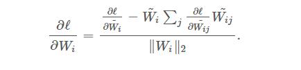
Or, we can directly use the standard back propagation to update $W$ and force to normalize it after each iteration. Which one is better still need examination by experiment.

Activation Layers

Relu

$E[y] = \sqrt {\frac{1}{2\pi}}$ and $Var[y] = \frac{1}{2}-\frac{1}{2\pi}$
so we should normalize the post-activation of ReLU by substracting
$\sqrt {\frac{1}{2\pi}}$ and dividing $\sqrt{\frac{1}{2}-\frac{1}{2\pi}}$

Sigmoid

$$E[y] = \frac{1}{2}$$
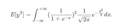
,I don’t think we can get a close form of the integral part of $E[y^2]$ Please note that we are not using the exact form of the equation. What we need is only an empirical value, so we can got the numbers by simulating.

we can get Sigmoid’s standard deviation: 0.2083. This value can be directly wrote into the program to let the post-sigmoid value have 1 standard deviation.

Pooling Layer

average-pooling

$E[y] = 0$and $Std[y]=\frac{1}{\sqrt{n}}=\frac{1}{s}$

max-pooling

The mean value of a 3×3 max-pooling is 1.4850 and the standard deviation is 0.5978. For 2×2 max-pooling, mean is 1.0291 and standard deviation is 0.7010.

Dropout Layer

Dropout is also a widely used layer in CNN. Although it is claimed to be useless in the NormProp paper, we still would like to record the formulations here. Dropout randomly erase values with a probability of 1−p.
Interestingly, this result is different from what we usually do. We usally preserve values with a ratio of p and divide the preserved values by p too. Now as we calculated, to achieve 1 s.t.d., we should divide the preserved values by $\sqrt{p}$. This result should be carefully examined by experiment in the future.

Conculsion

We believe that normalizing every layer with mean substracted and s.t.d. divided will become a standard in the near future. Now we should start to modify our present layers with the new normalization method, and when we are creating new layers, we should keep in mind to normalzie it with the method introduced above.

The shortage of this report is that we haven’t considered the back-propagation procedure. In paper[1][2], they claim that by normalizing the singular values of Jacobian matrix to 1 will lead to faster convergency and more numerically stable.

Reference

[1] Devansh Arpit, Yingbo Zhou, Bhargava U. Kota, Venu Govindaraju, Normalization Propagation: A Parametric Technique for Removing Internal Covariate Shift in Deep Networks. http://arxiv.org/abs/1603.01431
[2] Andrew M. Saxe, James L. McClelland, Surya Ganguli, Exact solutions to the nonlinear dynamics of learning in deep linear neural networks. http://arxiv.org/abs/1312.6120