聚类实验分析（KMeans,DBSCAN,图片分割,解决半监督问题,评估方法,K值选取）

乔大将军

已于 2024-02-19 22:49:02 修改

阅读量787

点赞数 14

分类专栏：机器学习文章标签：聚类机器学习人工智能 python

于 2024-02-18 16:46:20 首次发布

本文链接：https://blog.csdn.net/JamesSwifte/article/details/136152562

版权

机器学习专栏收录该内容

24 篇文章 3 订阅

订阅专栏

2、说明

1. 可以查看不同K值对应的inertia_，查看拐点

1、前言

在阅读本文前需要了解聚类算法的原理，可以参考聚类算法理论篇(K-means,DBSCAN原理)，聚类算法(K-means)代码实现(鸢尾花数据集)。

本文主要分析：

1.KMeans和DBSCAN算法

2. KMeans的评估方法和K值选取1

2. 聚类算法用于图像分割

3. 聚类算法可用于解决半监督问题

4. 聚类的评估方法。

2、说明

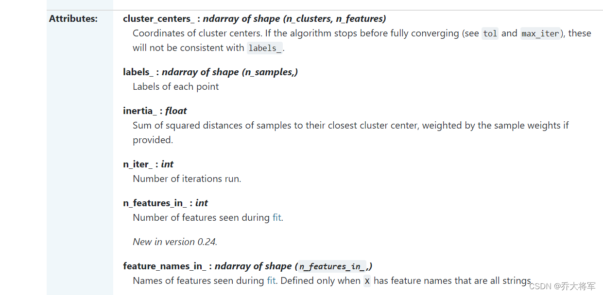
本文实验分析采用的是自作的数据集、手写数字数据集，采用python==3.9编译环境，机器学习包sklearn==1.4版本。对于文章代码中的一些机器学习类的属性，调用参数不懂可以参考：scikit-learn文档。用法已在模型的评估方法中说明。

3、实验分析

3.1 导入包

#导入包
import os
import numpy as np
import matplotlib
%matplotlib inline
import matplotlib.pyplot as plt
plt.rcParams['axes.labelsize'] = 14
plt.rcParams['xtick.labelsize'] = 12
plt.rcParams['ytick.labelsize'] = 12
import warnings
warnings.filterwarnings('ignore')

3.2 构造需要聚类的数据

#构造数据
from sklearn.datasets import make_blobs
blob_centers = np.array([[0.2,2.3],
                        [-1.5,2.3],
                        [-2.8,1.8],
                        [-2.8,2.8],
                        [-2.8,1.3]]) #表示5个簇的中心点，用它们去发散
blob_std = np.array([0.4,0.3,0.1,0.1,0.1]) #发散的程度
X,y = make_blobs(n_samples=2000,centers=blob_centers,cluster_std=blob_std,random_state=7)

#查看数据
def plot_clusters(X,y=None):
    plt.scatter(X[:,0],X[:,1],c=y,s=1)
    plt.xlabel("$x_1$",fontsize = 14)
    plt.ylabel("$x_2$",fontsize = 14,rotation=0)

plt.figure(figsize=(8,4))
plot_clusters(X)
plt.show()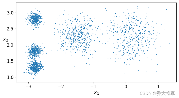

3.3 了解使用KMeans

看出上面的数据集，可以使用KMeans算法聚类，可以聚为5类或者4类或者n类，即K值需要自己设置。为了便于观察，绘制出决策边界。

#1决策边界
from sklearn.cluster import KMeans
k = 4 #假装知道k值
kmeans = KMeans(n_clusters=k,random_state=42)
y_pred = kmeans.fit_predict(X)

print(y_pred[:10]) #表示样本所属的簇类
print(kmeans.cluster_centers_) #表示质心点的位置

print(kmeans.labels_[:10] )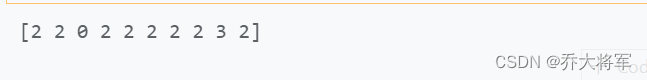

可以看出fit_predict(X)和kmeans.labels_d得到的结果是一样的，介绍一下KMeans的属性功能。

做出预测：

#预测
X_new = np.array([[0,2],[3,2],[-3,3],[-3,2.5]])
print(kmeans.predict(X_new))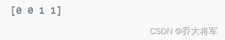

绘制聚类结果：

#2聚类结果展示
def plot_data(X):
    plt.plot(X[:,0],X[:,1],'k.',markersize=2)

def plot_centroids(centroids,weights=None,circle_color='w',cross_color='k'):
    if weights is not None:
        centroids = centroids[weights > weights.max() /10]
    plt.scatter(centroids[:,0],centroids[:,1],
                marker='o',s=10,linewidths=10,
                color=circle_color,zorder=10,alpha=0.9)
    plt.scatter(centroids[:,0],centroids[:,1],
                marker='x',s=20,linewidths=1,
                color=cross_color,zorder=11,alpha=1)
    
def plot_decision_boundaries(clusterer,X,resolution=1000,show_centroids=True,
                             show_xlabels=True,show_ylabels=True):
    mins = X.min(axis=0) - 0.1
    maxs = X.max(axis=0) + 0.1
    xx,yy = np.meshgrid(np.linspace(mins[0],maxs[0],resolution),
                        np.linspace(mins[1],maxs[1],resolution))
    #print(xx.max())
    #print(xx.min())
    #print(yy.max())
    #print(yy.min())
    Z = clusterer.predict(np.c_[xx.ravel(),yy.ravel()])
    Z = Z.reshape(xx.shape)

    plt.contourf(Z,extent=(mins[0],maxs[0],mins[1],maxs[1]),cmap='Pastel2') #绘制区域颜色
    plt.contour(Z,extent=(mins[0],maxs[0],mins[1],maxs[1]),linewidths = 1,colors = 'k')
    plot_data(X)
    if show_centroids:
        #print(clusterer.cluster_centers_)
        plot_centroids(clusterer.cluster_centers_)
    if show_xlabels:
        plt.xlabel("$x_1$",fontsize = 14)
    else:
        plt.tick_params(labelbottom='off')
    if show_ylabels:
        plt.ylabel("$x_2$",fontsize = 14,rotation=0)
    else:
        plt.tick_params(labelleft='off')


plt.figure(figsize=(8,4))
plot_decision_boundaries(kmeans,X)
plt.show()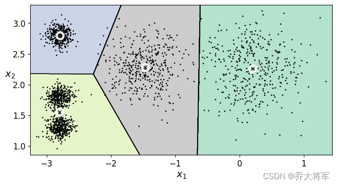

3.4 算法流程

知道KMeans算法的同学都知道，算法的工作流程：

1.根据K值，随机创建K个初始化质心点（Initialozation Randomly selecr K center points。

2. 算出所有样本点到质心点的距离，得到样本属于那个簇。

3. 更新，根据簇内样本重新算出簇内的质心。

4. 重复执行2，3步，重新划分簇类，直至质心不在变化。

#3算法流程 分别迭代1，2，3次随机种子保持一致，确保初始值相同
kmeans_iter1 = KMeans(n_clusters = 4,init = 'random',n_init =1 ,max_iter =1 ,random_state =1 )
kmeans_iter2 = KMeans(n_clusters = 4,init = 'random',n_init =1 ,max_iter =2 ,random_state =1 )
kmeans_iter3 = KMeans(n_clusters = 4,init = 'random',n_init =1 ,max_iter =3 ,random_state =1 )
kmeans_iter1.fit(X)
kmeans_iter2.fit(X)
kmeans_iter3.fit(X)
plt.figure(figsize=(12,8))
plt.subplot(321)
plot_data(X)
plot_centroids(kmeans_iter1.cluster_centers_,circle_color='r',cross_color='k')
plt.title('updata cluster_centers')
plt.subplot(322)
plot_decision_boundaries(kmeans_iter1,X)
plt.title('labels')
plt.subplot(323)
plot_decision_boundaries(kmeans_iter1,X,show_centroids=False)
plot_centroids(kmeans_iter2.cluster_centers_,circle_color='r',cross_color='k')
plt.title('updata cluster_centers')
plt.subplot(324)
plot_decision_boundaries(kmeans_iter2,X)
plt.title('labels')
plt.subplot(325)
plot_decision_boundaries(kmeans_iter2,X,show_centroids=False)
plot_centroids(kmeans_iter3.cluster_centers_,circle_color='r',cross_color='k')
plt.title('updata cluster_centers')
plt.subplot(326)
plot_decision_boundaries(kmeans_iter3,X)
plt.title('labels')
plt.show()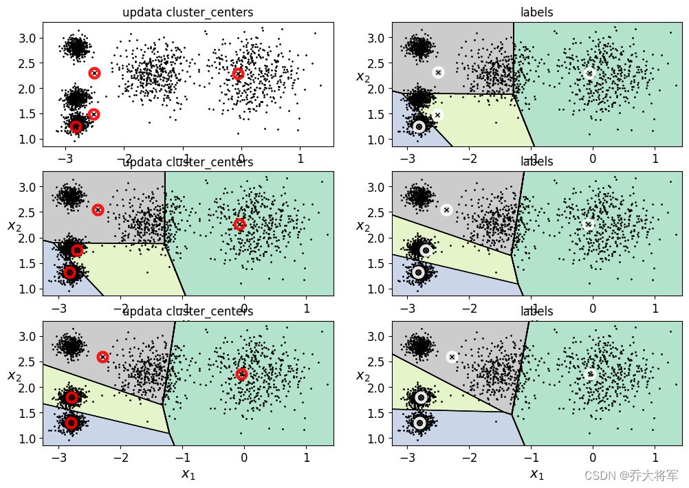

3.5 KMeans的不稳定性

KMeans具有不稳定的缺点，和参数K，质心初始值有很大关系

#4不稳定的结果
def plot_cluster_comparsion(c1,c2,X):
    c1.fit(X)
    c2.fit(X)
    plt.figure(figsize=(12,4))
    plt.subplot(121)
    plot_decision_boundaries(c1,X)
    plt.subplot(122)
    plot_decision_boundaries(c2,X)

c1 = KMeans(n_clusters=4,init='random',n_init=1,random_state=11)
c2 = KMeans(n_clusters=4,init='random',n_init=1,random_state=19)
plot_cluster_comparsion(c1,c2,X)
plt.show()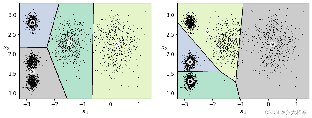

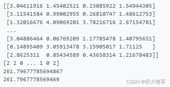
3.6 评估指标

我们知道由于数据集没有标签，很难去评判算法的优劣性，但对于KMeans算法来说，可以用inertia_:

float Sum of squared distances of samples to their closest cluster center, weighted by the sample weights if provided.即每个样本与其质心的距离越小越好。

#5评估指标
print(kmeans.inertia_)
x_dist = kmeans.transform(X) #样本到每个质心的距离
print(x_dist)

print(kmeans.labels_)
#x_dist[np.array(len(x_dist),kmeans.labels_)]
print(np.sum(x_dist[np.arange(len(x_dist)),kmeans.labels_]**2))
print(-kmeans.score(X))

3.7 找到合适的K值

1. 可以查看不同K值对应的inertia_，查看拐点

#6 如何去找到合适的K值 如果k值越大，得到的结果肯定越来越小
k_means_per_k = [KMeans(n_clusters = k).fit(X) for k in range(1,10)]
inertias = [model.inertia_ for model in k_means_per_k]
plt.figure(figsize=(8,4))
plt.plot(range(1,10),inertias,'bo-')
plt.show() #拐点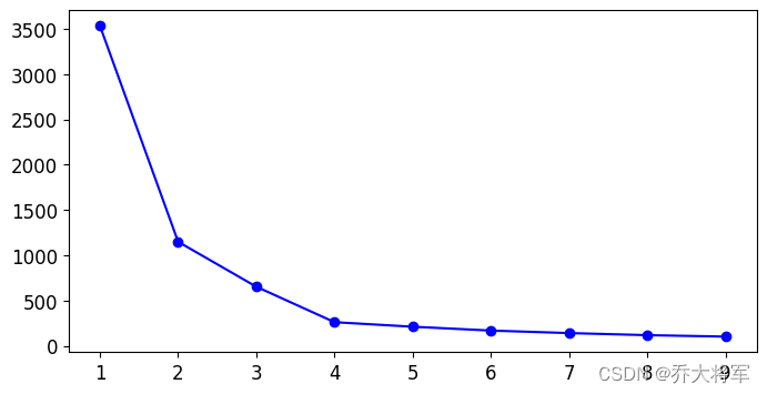

2. 轮廓系数

$a_i$ : 计算样本 $i$ 到同簇其他样本的平均距离 $a_i$ ， $a_i$ 越小，说明样本i越应该聚类到该簇；将 $a_i$ 称为样本 $i$ 的簇内不相似度。

$b_i$ ：计算样本 $i$ 到其他某簇 $c_j$ 的所有样本的平均距离 $b_{ij}$ ，称为样本 $i$ 与簇 $c_j$ 的不相似度。定义为样本 $i$ 的簇间不相似度。

$b_i = min(b_{i1},b_{i2},...,b_{ik})$

$s_i = \frac{b_{(i)}-a_{(i)}}{max({a_{(i)},b_{(i)}})}$

$s_i=\left\{\begin{matrix} 1-\frac{a_{(i)}}{b_{(i)}}, a_{(i)} < b_{(i)}\\ 0, a_{(i)} = b_{(i)}\\ \frac{b_{(i)}}{a_{(i)}} - 1,a_{(i)} > b_{(i)}\\ \end{matrix}\right.$

结论： $s_i$ 越接近于1，则说明样本i聚类合理

$s_i$ 越接近于-1，则说明样本i更应该聚类到其他簇类

$s_i$ 越接近于0，则说明样本i在两簇的边界上


from sklearn.metrics import silhouette_score #轮廓系数
#silhouette_score(X,kmeans.labels_)
silhouette_scores = [silhouette_score(X,model.labels_) for model in k_means_per_k[1:]]
plt.figure(figsize=(8,4))
plt.plot(range(2,10),silhouette_scores,'bo-')
plt.show() #拐点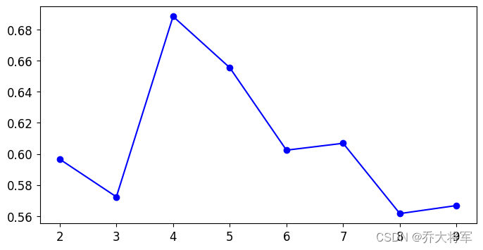

3.8 kmeas存在的问题

评估标准只作为参考 ,重新构造数据集

#8kmeas存在的问题 评估标准只作为参考
X1,y1 = make_blobs(n_samples=1000,centers=((4,-4,),(0,0)),random_state=42)
X1 = X1.dot(np.array([[0.374,0.95],[0.732,0.598]]))
X2,y2 = make_blobs(n_samples=250,centers = 1,random_state=42)
X2 = X2 + [6,-8]
X = np.r_[X1,X2]
y = np.r_[y1,y2]
plot_data(X)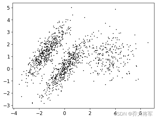

kmeans_good = KMeans(n_clusters=3,init=np.array([[-1.7,1.2],[0,0],[3.8,1]]),n_init=1,random_state=42) #玩赖
kmeans_bad = KMeans(n_clusters=3,random_state=42)
kmeans_good.fit(X)
kmeans_bad.fit(X)
plt.figure(figsize=(10,4))
plt.subplot(121)
plot_decision_boundaries(kmeans_good,X)
plt.title('kmeans_good inertia ={}'.format(kmeans_good.inertia_))
plt.subplot(122)
plot_decision_boundaries(kmeans_bad,X)
plt.title('kmeans_bad inertia ={}'.format(kmeans_bad.inertia_))
plt.show()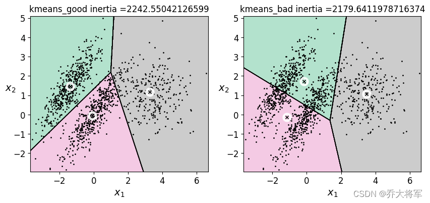

可以看到好的分类结果的inertia_值要大于不好的分类结果，所以只做参考，不能全信，多做实验。

3.9 图像分割小例子

图片读者复现时可以自选。

#9图像分割小实验
from matplotlib.image import imread
image = imread('book.jpg')
print(image.shape) #长，宽，3个颜色通道
X = image.reshape(-1,3) # 输入的数据n_samples * n_features -1: 439*658*3/3
print(X.shape)

kmeans = KMeans(n_clusters=6,random_state=42).fit(X)
print(kmeans.cluster_centers_)
print(kmeans.labels_)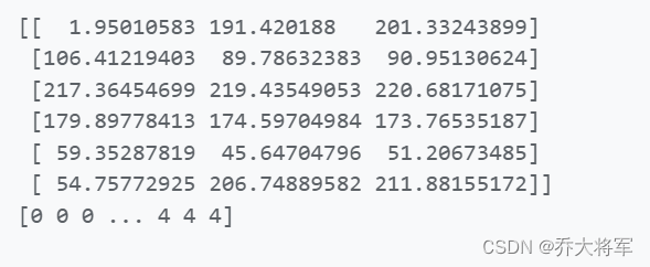

#segmented_img = kmeans.cluster_centers_[kmeans.labels_].reshape(439,658,3)
segmented_imgs = []
n_colors = (10,8,6,4,2)
for n_cluster in n_colors:
    kmeans = KMeans(n_clusters=n_cluster,random_state=42).fit(X)
    segmented_img =  segmented_img = kmeans.cluster_centers_[kmeans.labels_]
    segmented_imgs.append(segmented_img.reshape(image.shape)) #转换成长*宽*3
#plt.imshow(segmented_imgs[0].astype(float) / 255)
plt.figure(figsize=(10,5))
plt.subplot(231)
plt.imshow(image)
plt.title('original image')
for idx,n_clusters in enumerate (n_colors):
    plt.subplot(232+idx)
    plt.imshow(segmented_imgs[idx].astype(float) / 255)
    plt.title('{} colors'.format(n_clusters))
#plt.show()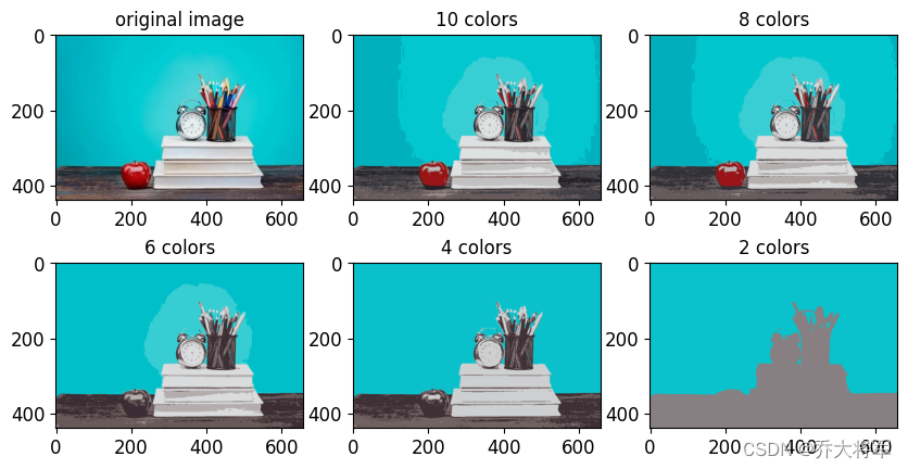

3.10 用于半监督学习

聚类也可以用来给无标签的数据打上标签，实现半监督学习。我们这里采用手写数字识别，实现10分类。

#10半监督学习，聚类也可以用来给无标签的数据打上标签，实现半监督学习
#导入数据
from sklearn.datasets import load_digits
X_digits,y_digits = load_digits(return_X_y=True)
from sklearn.model_selection import train_test_split
X_train,X_test,y_train,y_test = train_test_split(X_digits,y_digits,random_state=42)
print(X_train.shape)

#先用逻辑回归测试 10分类
from sklearn.linear_model import LogisticRegression
n_labels = 50  #只训练50个样本
log_reg = LogisticRegression(random_state=42)
log_reg.fit(X_train[:n_labels],y_digits[:n_labels])
print(log_reg.score(X_test,y_test))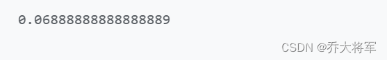

训练效果并不好。

用KMeans实现半监督学习，首先我们将训练数据集聚类为50个集群，然后对于每个聚类，让我们找到最靠近质心的图像，把这个图像称为代表性图像。

#假装原数据没有标签
#把图像聚类为50个，找到最近质心的图像，称为代表性图像
k = 50
kmeans = KMeans(n_clusters=k,random_state=42)
X_digits_dist = kmeans.fit_transform(X_train) #得出所有样本到各自簇内的距离
representation_digits_idx = np.argmin(X_digits_dist,axis=0) #最近的那个图像的索引
print(representation_digits_idx)
X_representation_digits = X_train[representation_digits_idx] #最近的那个图像
#print(X_representation_digits)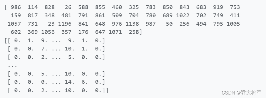

#展示这些图像
plt.figure(figsize=(8,2))
for index,X_representation_digit in enumerate(X_representation_digits):
    plt.subplot(k//10,10,index+1)
    plt.imshow(X_representation_digit.reshape(8,8),cmap='binary',interpolation='bilinear')
    plt.axis('off')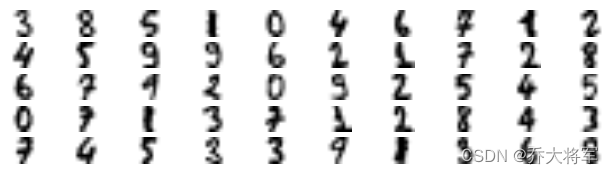

#手动打标签
y_representation_digits = np.array([
    3,8,5,1,0,4,6,9,1,2,
    4,5,9,9,6,2,2,7,2,8,
    6,7,7,2,0,9,2,5,4,5,
    0,7,1,3,7,2,2,8,4,3,
    7,4,5,3,3,9,1,3,6,8
])

#现在我们有了一个有50个标签的实列，它们每一个都是其集群的代表图像，而不是完全随机的实列，看看效果是否会更好
log_reg = LogisticRegression(random_state=42)
log_reg.fit(X_representation_digits,y_representation_digits)
log_reg.score(X_test,y_test)

可以看到，效果有显著提升。

一些扩展：

#标签传播，将每个簇内的所有实例打上和代表性图像一样的标签
y_train_propataged = np.empty(len(y_train),dtype=np.int32)
for i in range(k):
    y_train_propataged[kmeans.labels_ == i] = y_representation_digits[i]

log_reg = LogisticRegression(random_state=42)
log_reg.fit(X_train,y_train_propataged)
log_reg.score(X_test,y_test)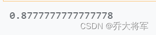

#只用每个簇的前20个做训练
percentile_closet = 20
X_cluster_dist = X_digits_dist[np.arange(len(X_train)),kmeans.labels_]
for i in range(k):
    in_cluster = (kmeans.labels_ == i)
    cluster_dist = X_cluster_dist[in_cluster] #选择属于当前簇的所有样本
    cutoff_distance = np.percentile(cluster_dist,percentile_closet) #排序找到前20个
    above_cutoff = (X_cluster_dist > cutoff_distance) # Fasle or True
    X_cluster_dist[in_cluster & above_cutoff] = -1 #在当前簇内，但是没在前20个
    partially_protaged = (X_cluster_dist != -1)
    X_train_partially_protagated = X_train[partially_protaged]
    y_train_partially_protagated = y_train_propataged[partially_protaged]
log_reg = LogisticRegression(random_state=42)
log_reg.fit(X_train_partially_protagated,y_train_partially_protagated)
log_reg.score(X_test,y_test)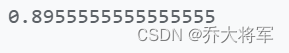

3.11 DBSCAN算法

DBSCAN算法是比KMeans应用更加广泛的算法，读者应该掌握。

重新构造数据集。

from sklearn.datasets import make_moons
X,y = make_moons(n_samples=1000,noise=0.05,random_state=42)
plt.plot(X[:,0],X[:,1],'b.')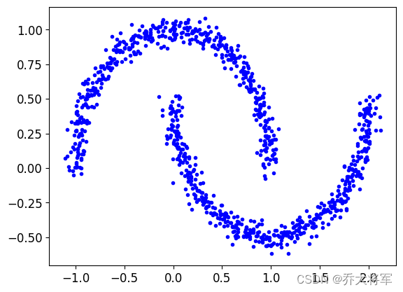

from sklearn.cluster import DBSCAN
dbscan = DBSCAN(eps=0.05,min_samples=5)
dbscan.fit(X)
print(dbscan.labels_[:10]) #每个样本所属簇类，这个算法不需要K值
print(dbscan.core_sample_indices_[:10]) #核心点
print(np.unique(dbscan.labels_))
dbscan_comparsion = DBSCAN(eps=0.2,min_samples=5)
dbscan_comparsion.fit(X)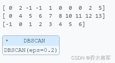

绘制图形

def plot_dbscan(dbscan,X,size,show_xlabels = True,show_ylabels=True):
    core_mask = np.zeros_like(dbscan.labels_,dtype=bool)
    core_mask[dbscan.core_sample_indices_] = True # 核心对象
    anomalies_mask = dbscan.labels_ == -1 # 离群点
    non_core_mask = ~(core_mask | anomalies_mask) # 普通点
    cores = dbscan.components_
    anomalies = X[anomalies_mask]
    non_core = X[non_core_mask]
    plt.scatter(cores[:,0],cores[:,1],c = dbscan.labels_[core_mask],marker = 'o', s = size,cmap='Paired')
    plt.scatter(cores[:,0],cores[:,1],c = dbscan.labels_[core_mask],marker = '*', s = 20)
    plt.scatter(anomalies[:,0],anomalies[:,1],c = 'r',marker = 'x', s = 100)
    plt.scatter(non_core[:,0],non_core[:,1],c  = dbscan.labels_[non_core_mask],marker = '.')
    if show_xlabels:
        plt.xlabel("$x_1$",fontsize = 14)
    else:
        plt.tick_params(labelbottom='off')
    if show_ylabels:
        plt.ylabel("$x_2$",fontsize = 14,rotation=0)
    else:
        plt.tick_params(labelleft='off')
    plt.title('eps = {:.2f} minsamples = {}'.format(dbscan.eps,dbscan.min_samples),fontsize = 14)

plt.figure(figsize=(9,4))
plt.subplot(121)
plot_dbscan(dbscan,X,size=100)
plt.subplot(122)
plot_dbscan(dbscan_comparsion,X,size=600,show_ylabels=False)

plt.show()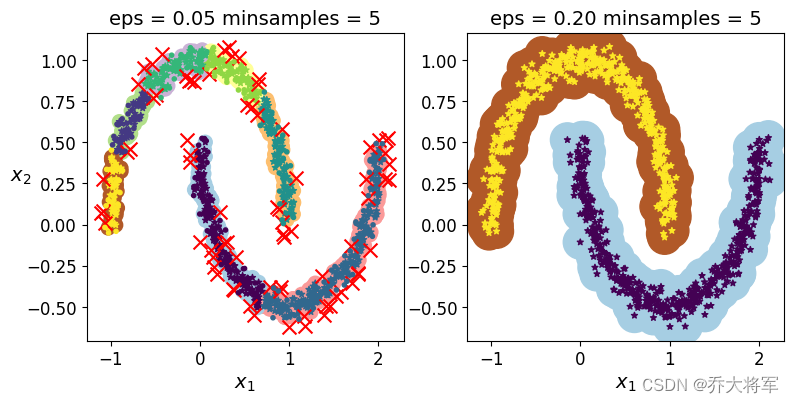

可以看出两个参数eps(半径)，min_samples(阈值)对于结果的影响很大，左上分为6个簇，而事实是两个簇。找到合适的参数需得多做实验。

乔大将军

关注

14
点赞
踩
17

收藏

觉得还不错? 一键收藏
0
评论
聚类实验分析（KMeans,DBSCAN,图片分割,解决半监督问题,评估方法,K值选取）

在阅读本文前需要了解聚类算法的原理，可以参考聚类算法理论篇(K-means,DBSCAN原理)聚类算法(K-means)代码实现(鸢尾花数据集)。本文主要分析：1.KMeans和DBSCAN算法2. KMeans的评估方法和K值选取12. 聚类算法用于图像分割3. 聚类算法可用于解决半监督问题4. 聚类的评估方法。
复制链接

扫一扫