n3_knn breastCancer NaiveBayesLikelihood_voter_manhat_Euclid_Minkow_空值?_SBS特征选取_Laplace_zip_NLP_spam

     In the n2_Tree ML Models_HR data_Chi-square_SAMME_AdaBoost_GradientBoosting_XGBoost_class weight_Ensemble_Linli522362242的专栏-CSDN博客, we have learned about computationally intensive methods. In contrast, this chapter discusses the simple methods to balance it out! We will be covering the two techniques, called k-nearest neighbors (KNN)and Naive Bayes here. Before touching on KNN, we explained the issue with the curse of dimensionality with a simulated example. Subsequently, breast cancer medical examples have been utilized to predict whether the cancer is malignant or benign using KNN. In the final section of the chapter, Naive Bayes has been explained with spam/ham classification, which also involves the application of the natural language processing (NLP) techniques consisting of the following basic preprocessing and modeling steps:

• Punctuation removal
• Word tokenization and lowercase conversion
• Stopwords removal
• Stemming
• Lemmatization with POS tagging Conversion of words into TF-IDF to create numerical representation of words Application of the Naive Bayes model on TF-IDF vectors to predict if the message is either spam or ham on both train and test data

K-nearest neighbors

     K-nearest neighbors is a non-parametric machine learning model in which the model memorizes the training observation for classifying the unseen test data. It can also be called instance-based learning. This model is often termed as lazy learning, as it does not learn anything during the training phase like regression, random forest, and so on. Instead, it starts working only during the testing/evaluation phase to compare the given test observations with the nearest training observations, which will take significant time in comparing each test data point. Hence, this technique is not efficient on big data; also, performance does deteriorate[dɪˈtɪriəreɪt]恶化 when the number of variables is high due to the curse of dimensionality.

KNN voter example

     KNN is explained better with the following short example. The objective is to predict the party for which voter will vote based on their neighborhood社区, precisely geolocation (latitude and longitude). Here we assume that we can identify the potential voter to which political party they would be voting based on majority voters did vote for that particular party in that vicinity[vəˈsɪnəti]周围地区 so that they have a high probability to vote for the majority party. However, tuning the k-value (number to consider, among which majority should be counted) is the million-dollar question (as same as any machine learning algorithm):

     In the preceding diagram, we can see that the voter of the study will vote for Party 2. As within the vicinity, one neighbor has voted for Party 1 and the other voter voted for Party 3. But three voters voted for Party 2. In fact, by this way, KNN solves any given classification problem. Regression problems are solved by taking mean of its neighbors within the given circle or vicinity or k-value.

Curse of dimensionality维度诅咒

     KNN completely depends on distance. Hence, it is worth studying about the curse of dimensionality to understand when KNN deteriorates[dɪˈtɪriəreɪt]恶化 its predictive power with the increase in the number of variables required for prediction. This is an obvious fact that high-dimensional spaces are vast. Points in high-dimensional spaces tend to be dispersing[dɪ'spɜːrs]分散的 使散开 from each other more compared with the points in low-dimensional space. Though there are many ways to check the curve of dimensionality, here we are using uniform random values between zero and one generated for 1D, 2D, and 3D space to validate this hypothesis.

     In the following lines of codes, the mean distance between 1,000 observations has been calculated with the change in dimensions. It is apparent that with the increase in dimensions, distance between points increases logarithmically, which gives us the hint that we need to have an exponential increase in data points with increase in dimensions in order to make machine learning algorithms work correctly:

import numpy as np
import pandas as pd

# KNN Curse of Dimensionality
import random, math

     The following code generates random numbers between zero and one from uniform distribution with the given dimension, which is equivalent of length of array or list:

def random_point_gen( dimension ): 
    # random.random() : Return random number between 0.0 and 1.0
    return [random.random() for _ in range( dimension )]

     The following function calculates root mean sum of squares of Euclidean distances (2-
norm) between points by taking the difference between points and sum the squares and finally takes the square root of total distance:

def distance( v, w ):
    vec_sub = [ v_i-w_i for v_i, w_i in zip(v,w) ]
    sum_of_sqrs = sum( v_i*v_i for v_i in vec_sub )
    
    return math.sqrt( sum_of_sqrs )

     Both dimension and number of pairs are utilized for calculating the distances with the following code:

def random_distances_comparison( dimension, number_pairs ):
             # 2D data points   
    return [ distance( random_point_gen(dimension), 
                       random_point_gen(dimension)
                     ) for _ in range( number_pairs )
           ]

def mean(x):
    return sum(x)/len(x)

     The experiment has been done by changing dimensions from 1 to 201 with an increase of 5 dimensions to check the increase in distance:

dimensions = range(1, 201, 5) # step=5

     Both minimum and average distances have been calculated to check, however, both illustrate the similar story:

avg_distances = []
min_distances = []

dummyarray = np.empty( (20,4) ) # uninitialized
dist_vals = pd.DataFrame( dummyarray )
dist_vals.columns = ['Dimension', 'Min_Distance', 'Avg_Distance', 'Min/Avg_Distance']

dist_vals

random.seed(34)
row_index = 0
for dims in dimensions:
                                        # sqrt( sum( square(difference), axis=1 ) )
    distances = random_distances_comparison( dims, number_pairs=1000 )
    avg_distances.append( mean(distances) )
    min_distances.append( min(distances) )
    
    dist_vals.loc[row_index, 'Dimension'] = dims
    dist_vals.loc[row_index, 'Min_Distance'] = np.min(distances)
    dist_vals.loc[row_index, 'Avg_Distance'] = np.mean(distances)
    dist_vals.loc[row_index, 'Min/Avg_Distance'] = min(distances)*1.0/mean(distances)
    row_index +=1
    
dist_vals

 
Plotting Average distances for Various Dimensions

import matplotlib.pyplot as plt

fig = plt.figure( figsize=(10,8) )

plt.xlabel( 'Dimensions', fontsize=14 )
plt.ylabel( 'Avg. Distance', fontsize=14 )

plt.plot( dist_vals['Dimension'], dist_vals['Avg_Distance'], label='Avg_Distance' )
plt.legend( loc='best' )

plt.show()

  VS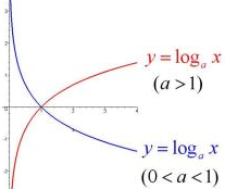
     From the preceding graph, it is proved that with the increase in dimensions, mean distance increases logarithmically. Hence the higher the dimensions, the more data is needed to overcome the curse of dimensionality!（Disadvantages of knn, Besides,The only deficiency of KNN classifier would be, it is computationally intensive计算量很大 during test phase, as each test observation will be compared with all the available observations in train data, which practically KNN does not learn a thing from training data. Hence, we are also calling it a lazy classifier!）

Curse of dimensionality with 1D, 2D, and 3D example

      A quick analysis has been done to see how distance 60 random points are expanding with the increase in dimensionality. Initially, random points are drawn for one-dimension:

# 1-Dimension Plot
import numpy as np
import pandas as pd
import matplotlib.pyplot as plt

             # random samples from a uniform distribution over [0, 1)
one_dim_data = np.random.rand(60,1)
one_dim_data_df = pd.DataFrame( one_dim_data )
one_dim_data_df.columns = ['1D_Data']
one_dim_data_df['height'] = 1

one_dim_data_df.head(n=5)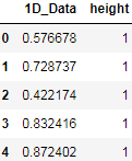

 

plt.figure( figsize=(10,6) )

plt.scatter( one_dim_data_df['1D_Data'], one_dim_data_df['height'] )

plt.title( '60 Random Points Generated on 1-D', color='red', 
           fontsize=20, fontstyle='italic', fontweight = 'medium',
           family='sans-serif'
         )
plt.yticks([])
plt.xlabel('1-D points', fontsize=14 )

plt.show()

If we observe the following graph, all 60 data points are very nearby in one-dimension: 
     Here we are repeating the same experiment in a 2D space, by taking 60 random numbers with x and y coordinate space and plotted them visually:

# 2- Dimensions Plot

two_dim_data = np.random.rand(60,2)
two_dim_data_df = pd.DataFrame(two_dim_data)
two_dim_data_df.columns = ['x_axis', 'y_axis']

plt.figure( figsize=(10,6) )

plt.scatter( two_dim_data_df ['x_axis'], two_dim_data_df ['y_axis'] )
plt.title( '60 Random Points Generated on 2-D', color='red', 
           fontsize=20, fontstyle='italic', fontweight = 'medium',
           family='serif'
         )

plt.xlabel( 'x_axis' , fontsize=14 )
plt.ylabel( 'y_axis' , fontsize=14 )

plt.show()

     By observing the 2D graph we can see that more gaps have been appearing for the same 60
data points:
     Finally, 60 data points are drawn for 3D space. We can see a further increase in spaces, which is very apparent. This has proven to us visually by now that with the increase in dimensions, it creates a lot of space, which makes a classifier weak to detect the signal:

# 3-Dimensions Plot

three_dim_data = np.random.rand(60,3)
three_dim_data_df = pd.DataFrame( three_dim_data )
three_dim_data_df.columns = ['x_axis', 'y_axis', 'z_axis']

from mpl_toolkits.mplot3d import Axes3D

fig = plt.figure( figsize=(10,8) )
ax = fig.add_subplot(111, projection='3d')

plt.title( '60 Random Points Generated on 3-D', color='red', 
           fontsize=20, fontstyle='italic', fontweight = 'medium'
         )
ax.scatter( three_dim_data_df['x_axis'], 
            three_dim_data_df['y_axis'],
            three_dim_data_df['z_axis']
          )
plt.show()

 

KNN classifier with breast cancer Wisconsin data example

     Breast cancer data has been utilized from the UCI machine learning repository UCI Machine Learning Repository: Breast Cancer Wisconsin (Diagnostic) Data Set for illustration purposes. Here the task is to find whether the cancer is malignant[məˈlɪɡnənt]恶性的  or benign[bɪˈnaɪn]良性的 based on various collected features such as clump[klʌmp] thickness 团块厚度and so on using the KNN classifier:
http://archive.ics.uci.edu/ml/machine-learning-databases/breast-cancer-wisconsin/breast-cancer-wisconsin.names

​​​​​​http://archive.ics.uci.edu/ml/machine-learning-databases/breast-cancer-wisconsin/breast-cancer-wisconsin.data

# KNN Classifier - Breast Cancer
import numpy as np
import pandas as pd
from sklearn.metrics import accuracy_score, classification_report

breast_cancer = pd.read_csv( 'http://archive.ics.uci.edu/ml/machine-learning-databases'
                             '/breast-cancer-wisconsin/breast-cancer-wisconsin.data',
                             names = ['ID_Number','Clump_Thickness', 'Uniformity of Cell Size',
                                        'Uniformity_of_Cell_Shape', 'Marginal_Adhesion',
                                        'Single_Epithelial_Cell_Size', 'Bare_Nuclei',
                                        'Bland_Chromatin', 'Normal_Nucleoli',
                                        'Mitoses', 'Class'
                                       ]
                           )
breast_cancer

     The following are the few rows to show how the data looks like. The Class value has
class 2 and 4. Value 2 and 4 represent benign[bɪˈnaɪn]良性的 and malignant[məˈlɪɡnənt]恶性的 class, respectively. Whereas all the other variables do vary between value 1 and 10, which are very much categorical in nature:
​

 ​

breast_cancer.isnull().any()

 Is there really no null value?

breast_cancer.to_csv('Breast_Cancer_Wisconsin.csv')

  It is better to save it as a CSVfile and then open it with excel

breast_cancer.dtypes

 空值?

breast_cancer.isin(['?']).any()

 

      Only the Bare_Nuclei variable has some missing values, here we are replacing them with the most frequent value (category value 1) in the following code:

breast_cancer['Bare_Nuclei'] = breast_cancer['Bare_Nuclei'].replace('?', np.NAN)
breast_cancer.isnull().any()

breast_cancer['Bare_Nuclei'].value_counts()

 

breast_cancer['Bare_Nuclei'] = breast_cancer['Bare_Nuclei'].fillna( 
                    breast_cancer['Bare_Nuclei'].value_counts().index[0] 
                )
breast_cancer[20:25]

     Use the following code to convert the classes（The Class value has class 2 and 4. Value 2 and 4 represent benign[bɪˈnaɪn]良性的 and malignant[məˈlɪɡnənt]恶性的 class, respectively） to a 0 and 1 indicator for using in the classifier:

breast_cancer['Cancer_Ind'] = 0 # append a new column with name='Cancer_Ind' and values are equal to 0
breast_cancer.loc[ breast_cancer['Class']==4, 'Cancer_Ind' ] = 1
breast_cancer.head(n=6)

 In the following code, we are dropping non-value added variables from analysis:

x_vars = breast_cancer.drop( ['ID_Number', 'Class', 'Cancer_Ind'], 
                              axis=1 
                           )
y_var = breast_cancer['Cancer_Ind']

x_vars.head(n=6)

########################################### 

cp4 Training Sets Preprocessing_StringIO_dropna_categorical_feature_Encode_Scale_L1_L2_bbox_to_ancho_Linli522362242的专栏-CSDN博客

 min-max scaling VS standardization

     Now, there are two common approaches to bring different features onto the same scale: normalization and standardization. Those terms are often used quite loosely in different fields, and the meaning has to be derived from the context. Most often, normalization refers to the rescaling of the features to a range of [0, 1], which is a special case of min-max scaling. To normalize our data, we can simply apply the min-max scaling to each feature column, where the new value of a sample  can be calculated as follows: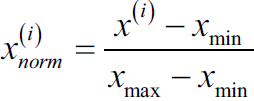Here,  is a particular sample,  is the smallest value in a feature column, and  the largest value

The min-max scaling procedure is implemented in scikit-learn and can be used as follows:

from sklearn.preprocessing import MinMaxScaler
 
mms = MinMaxScaler()
X_train_norm = mms.fit_transform(X_train)
X_test_norm = mms.transform(X_test)

    Although normalization via min-max scaling is a commonly used technique that is useful when we need values in a bounded interval, standardization can be more practical for many machine learning algorithms, especially for optimization algorithms such as gradient descent. The reason is that many linear models, such as the logistic regression and SVM that we remember from cp3, A Tour of Machine Learning Classifiers Using scikit-learncp3 sTourOfMLClassifiers_stratify_bincount_likelihood_logistic regression_odds ratio_decay_L2_sigmoi_Linli522362242的专栏-CSDN博客, initialize the weights to 0 or small random values close to 0. Using standardization, we center the feature columns at mean 0 with standard deviation 1 so that the feature columns takes the form of a normal distribution, which makes it easier to learn the weights. Furthermore, standardization maintains useful information about outliers and makes the algorithm less sensitive to them in contrast to min-max scaling, which scales the data to a limited range of values.

The procedure for standardization can be expressed by the following equation: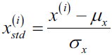

 Here,  is the sample mean of a particular feature column and  the corresponding standard deviation, respectively.
Please note that pandas uses ddof=1 (sample standard deviation) by default,
whereas NumPy's std method and the StandardScaler uses ddof=0 (population standard deviation)
cp1_Journey from Statistics to Machine Learning： https://blog.csdn.net/Linli522362242/article/details/91037961

 Numpy's std uses ddof=0 (population standard deviation)

     “Delta Degrees of Freedom”: the divisor used in the calculation is N - ddof, where N represents the number of elements. By default ddof is zero.

ex = np.array([0,1,2,3,4,5])
print( 'standardized:', ( ex - ex.mean() )/ex.std() )

( sum( (ex-ex.mean())**2 )/ ex.shape[0] )**0.5

 

ex.std()

==>Proved:Numpy's std uses ddof=0 (population standard deviation)

 Panda's std uses ddof=1 (sample standard deviation)

exDF=pd.DataFrame(ex)
print('standardized: ', 
      ( (exDF - exDF.mean())/ exDF.std() ).values.reshape(1, -1)[0]
     )

round( ( sum( (ex-ex.mean())**2 )/ (ex.shape[0]-1) )**0.5,
       6
     )

 

exDF.std()

==> Panda's std uses ddof=1 (sample standard deviation) 

print('normalized:', 
      ( ex-ex.min() )/( ex.max()-ex.min() )
     )

 

     Similar to the MinMaxScaler class, scikit-learn also implements a class for standardization:

uses ddof=0 (population standard deviation)

from sklearn.preprocessing import StandardScaler
stdsc = StandardScaler()
print( 'standardized:', 
      stdsc.fit_transform( ex.reshape(-1, 1) ).reshape(1,-1)[0] 
     )

 ########################################### 

from sklearn.preprocessing import StandardScaler

x_vars_stdscale = StandardScaler().fit_transform( x_vars.values )

 As KNN is very sensitive to distances, here we are standardizing all the columns before applying algorithms:

from sklearn.model_selection import train_test_split

x_vars_stdscale_df = pd.DataFrame( x_vars_stdscale, 
                                   index = x_vars.index,
                                   columns = x_vars.columns
                                 )
x_train, x_test, y_train, y_test = train_test_split( x_vars_stdscale_df,
                                                     y_var,
                                                     train_size=0.7,
                                                     random_state=42
                                                   )
x_train

  

p      int, default=2
        Power parameter for the Minkowski metric. When p = 1, this is equivalent to using manhattan_distance (l1), and euclidean_distance (l2) for p = 2. For arbitrary p, minkowski_distance (l_p) is used.
https://en.wikipedia.org/wiki/Minkowski_distance
The Minkowski distance of order p is an integer) between two points

is defined as: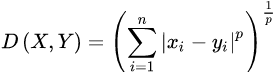

     KNN classifier is being applied with neighbor value of 3 and p value indicates it is 2-norm, also known as Euclidean distance for computing classes:

from sklearn.neighbors import KNeighborsClassifier

knn_fit = KNeighborsClassifier( n_neighbors=3, p=2, 
                                metric='minkowski'
                              )
knn_fit.fit( x_train, y_train )

print( '\nK-Nearest Neighbors - Train Confusion Matrix\n\n', 
       pd.crosstab( y_train, knn_fit.predict(x_train),
                    rownames=['Actuall'], colnames=['Predicted']
                  )
     )
print( '\nK-Nearest Neighbors - Train Accuracy: ',
       round( accuracy_score(y_train, knn_fit.predict(x_train) ),
              3
            )
     )
print( '\nK-Nearest Neightbors-Train Classification Report\n',
       classification_report( y_train, knn_fit.predict(x_train) )
     )

 

print( '\nK-Nearest Neighbors - Test Confusion Matrix\n\n', 
       pd.crosstab( y_test, knn_fit.predict(x_test),
                    rownames=['Actuall'], colnames=['Predicted']
                  )
     )
print( '\nK-Nearest Neighbors - Test Accuracy: ',
       round( accuracy_score(y_test, knn_fit.predict(x_test) ),
              3
            )
     )
print( '\nK-Nearest Neightbors-Test Classification Report\n',
       classification_report( y_test, knn_fit.predict(x_test) )
     )

 
     From the results, it is appearing that KNN is working very well in classifying malignant and benign classes well, obtaining test accuracy( =(TP+TN)/(TP+FP+FN+TN)=(64+141)/(64+141+3+2)) , Accuracy answers the following question: How many instances did we correctly label out of all the instances?) of 97.6 percent with 96 percent of recall( =TP/(TP+FN) = 64/( 3+64 ), Recall answers the following question: Of all the instances who are target class( cancer is malignant ), how many of those we correctly predict? ) on malignant class. The only deficiency of KNN classifier would be, it is computationally intensive during test phase, as each test observation will be compared with all the available observations in train data, which practically KNN does not learn a thing from training data. Hence, we are also calling it a lazy classifier!

Tuning of k-value in KNN classifier

     In the previous section, we just checked with only the k-value of three. Actually, in any machine learning algorithm, we need to tune the knobs to check where the better performance can be obtained. In the case of KNN, the only tuning parameter is k-value. Hence, in the following code, we are determining the best k-value with grid search:

# Tuning of K- value for Train & Test data

dummyarray = np.empty( (5,3) ) # 3 since ["K_value","Train_acc","Test_acc"]
k_valchart_df = pd.DataFrame( dummyarray ) #
k_valchart_df.columns = ["K_value","Train_acc","Test_acc"]

k_vals = [1,2,3,4,5]

for i in range( len(k_vals) ):
    knn_fit = KNeighborsClassifier( n_neighbors=k_vals[i],
                                    p = 2,
                                    metric = 'minkowski'
                                  )
    knn_fit.fit( x_train, y_train )
    
    print( '\nK-value', k_vals[i] )
    
    tr_accuracy = round( accuracy_score( y_train, knn_fit.predict(x_train) ),
                         3
                       )
    print( '\nK-Nearest Neighbors - Train Confusion Matrix\n\n', 
           pd.crosstab( y_train, knn_fit.predict( x_train ),
                        rownames = ['Actuall'], colnames=['Predicted']
                      )
         )
    print( '\nK-Nearest Neighbors - Train accuracy:', tr_accuracy )
    print( '\nK-Nearest Neighbors - Train Classification Report\n', 
           classification_report( y_train, knn_fit.predict(x_train) )
         )
    
    ts_accuracy = round( accuracy_score( y_test, knn_fit.predict(x_test) ),
                         3
                       )
    print( '\nK-Nearest Neighbors - Test Confusion Matrix\n\n', 
           pd.crosstab( y_test, knn_fit.predict( x_test ),
                        rownames = ['Actuall'], colnames=['Predicted']
                      )
         )
    print( '\nK-Nearest Neighbors - Test accuracy:', ts_accuracy )
    print( '\nK-Nearest Neighbors - Test Classification Report\n', 
           classification_report( y_test, knn_fit.predict(x_test) )
         )
    
    k_valchart_df.loc[i, 'K_value'] = k_vals[i]
    k_valchart_df.loc[i, 'Train_acc'] = tr_accuracy
    k_valchart_df.loc[i, 'Test_acc'] = ts_accuracy

 

 ... ...

Ploting accuracies over varied K-values

# Ploting accuracies over varied K-values
import matplotlib.pyplot as plt

plt.figure( figsize=(10,6) )
plt.xlabel( 'K-value' )
plt.ylabel( 'Accuracy' )
plt.plot( k_valchart_df['K_value'], k_valchart_df['Train_acc'], label='Train_acc' )
plt.plot( k_valchart_df['K_value'], k_valchart_df['Test_acc'], label='Test_acc', c='b')

plt.axis( [0.9, 5.5,
           0.92, 1.005
          ]
        )
plt.xticks( [1,2,3,4,5] )

for a,b in zip( k_valchart_df['K_value'], k_valchart_df['Train_acc'] ):
    plt.text( a,b, str(b), fontsize=10 )

for a,b in zip( k_valchart_df['K_value'], k_valchart_df['Test_acc'] ):
    plt.text( a,b, str(b), fontsize=10 )

plt.legend( loc='upper right' )
plt.show()

     It appears that with less value of k-value, it has more overfitting problems due to the very high value of accuracy on train data and less on test data, with the increase in k-value more the train and test accuracies are converging and becoming more robust. This phenomenon illustrates the typical machine learning phenomenon. As for further analysis, readers are encouraged to try k-values higher than five and see how train and test accuracies are changing.

# Tuning of K- value for Train & Test data

dummyarray = np.empty( (5,3) ) # 3 since ["K_value","Train_acc","Test_acc"]
k_valchart_df = pd.DataFrame( dummyarray ) #
k_valchart_df.columns = ["K_value","Train_acc","Test_acc"]

k_vals = [1,2,3,4,5, 6, 7, 8, 9, 10]

for i in range( len(k_vals) ):
    knn_fit = KNeighborsClassifier( n_neighbors=k_vals[i],
                                    p = 2,
                                    metric = 'minkowski'
                                  )
    knn_fit.fit( x_train, y_train )
    
    print( '\nK-value', k_vals[i] )
    
    tr_accuracy = round( accuracy_score( y_train, knn_fit.predict(x_train) ),
                         3
                       )
    print( '\nK-Nearest Neighbors - Train Confusion Matrix\n\n', 
           pd.crosstab( y_train, knn_fit.predict( x_train ),
                        rownames = ['Actuall'], colnames=['Predicted']
                      )
         )
    print( '\nK-Nearest Neighbors - Train accuracy:', tr_accuracy )
    print( '\nK-Nearest Neighbors - Train Classification Report\n', 
           classification_report( y_train, knn_fit.predict(x_train) )
         )
    
    ts_accuracy = round( accuracy_score( y_test, knn_fit.predict(x_test) ),
                         3
                       )
    print( '\nK-Nearest Neighbors - Test Confusion Matrix\n\n', 
           pd.crosstab( y_test, knn_fit.predict( x_test ),
                        rownames = ['Actuall'], colnames=['Predicted']
                      )
         )
    print( '\nK-Nearest Neighbors - Test accuracy:', ts_accuracy )
    print( '\nK-Nearest Neighbors - Test Classification Report\n', 
           classification_report( y_test, knn_fit.predict(x_test) )
         )
    
    k_valchart_df.loc[i, 'K_value'] = k_vals[i]
    k_valchart_df.loc[i, 'Train_acc'] = tr_accuracy
    k_valchart_df.loc[i, 'Test_acc'] = ts_accuracy

 

# Ploting accuracies over varied K-values
import matplotlib.pyplot as plt

plt.figure( figsize=(10,6) )
plt.xlabel( 'K-value' )
plt.ylabel( 'Accuracy' )
plt.plot( k_valchart_df['K_value'], k_valchart_df['Train_acc'], label='Train_acc', c='k' )
plt.plot( k_valchart_df['K_value'], k_valchart_df['Test_acc'], label='Test_acc', c='b')

plt.axis( [0.9, 10.5,
           0.92, 1.005
          ]
        )
plt.xticks( [1,2,3,4,5, 6, 7, 8, 9, 10] )

for a,b in zip( k_valchart_df['K_value'], k_valchart_df['Train_acc'] ):
    plt.text( a,b, str(b), fontsize=10, c='k' )

for a,b in zip( k_valchart_df['K_value'], k_valchart_df['Test_acc'] ):
    plt.text( a,b, str(b), fontsize=10, c='b' )

plt.legend( loc='upper right' )
plt.show()

 

k_valchart_df

 it is appearing that KNN is working very well in classifying malignant and benign classes well, obtaining test accuracy of 97.6 percent with 96 percent of recall on malignant class.

     However, please wait a moment, we seem to use all features. Can we further improve the performance of knn if we use feature selection?

Sequential feature selection algorithms

cp4 TrainingSetsPreprocessing_2_ Sequential feature selection_vs_Rand_tree_combinations_knn_format_%_Linli522362242的专栏-CSDN博客

    An alternative way to reduce the complexity of the model and avoid overfitting is dimensionality reduction via feature selection, which is especially useful for unregularized models. There are two main categories of dimensionality reduction techniques: feature selection and feature extraction. Using feature selection, we select a subset of the original features. In feature extraction, we derive information from the feature set to construct a new feature subspace. In this section, we will take a look at a classic family of feature selection algorithms. In the next chapter, Chapter 5, Compressing Data via Dimensionality Reduction, we will learn about different feature extraction techniques to compress a dataset onto a lower dimensional feature subspace.
cp5_Compressing Data via Dimensionality Reduction_feature extraction_PCA_LDA_convergence_kernel PCA:https://blog.csdn.net/Linli522362242/article/details/105196037

     In this section, we will take a look at a classic family of feature selection algorithms. In the next chapter, Chapter 5, Compressing Data via Dimensionality Reduction, we will learn about different feature extraction techniques to compress a dataset onto a lower-dimensional feature subspace.

     Sequential feature selection (for supervised learning) algorithms are a family of greedy search algorithms that are used to reduce an initial d-dimensional feature space to a k-dimensional feature subspace where k<d. The motivation behind feature selection algorithms is to automatically select a subset of features that are most relevant to the problem, to improve computational efficiency or reduce the generalization error of the model by removing irrelevant features or noise, which can be useful for algorithms that don't support regularization.

    A classic sequential feature selection algorithm is Sequential Backward Selection (SBS), which aims to reduce the dimensionality of the initial feature subspace with a minimum decay最小衰减 in performance of the classifier to improve upon computational efficiency. In certain cases, SBS can even improve the predictive power of the model if a model suffers from overfitting.

     The idea behind the SBS algorithm is quite simple: SBS sequentially removes features from the full feature subset until the new feature subspace contains the desired number of features. In order to determine which feature is to be removed at each stage, we need to define the criterion function J that we want to minimize. The criterion calculated by the criterion function can simply be the difference in performance of the classifier before and after the removal of a particular feature. Then, the feature to be removed at each stage can simply be defined as the feature that maximizes this criterion; or in more intuitive terms, at each stage we eliminate the feature that causes the least performance loss after removal. Based on the preceding definition of SBS, we can outline the algorithm in four simple steps:

• 1. Initialize the algorithm with k=d, where d is the dimensionality of the full feature space.
• 2. Determine the feature  that maximizes the criterion: 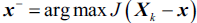, where .
• 3. Remove the feature  from the feature set: .
• 4. Terminate if k equals the number of desired features; otherwise, go to step 2.
   

     Unfortunately, the SBS algorithm has not been implemented in scikit-learn yet. But since it is so simple, let us go ahead and implement it in Python from scratch:

from sklearn.base import clone
from itertools import combinations
import numpy as np
from sklearn.metrics import accuracy_score
from sklearn.model_selection import train_test_split
 
class SBS():                      # k_features： minimum number of features
    def __init__(self, estimator, k_features, scoring=accuracy_score, test_size=0.3, 
                 random_state=42):
        self.scoring = scoring #criterion 
        self.estimator = clone(estimator)
        self.k_features = k_features
        self.test_size = test_size
        self.random_state = random_state
                                                            # indices : feature_index_list
    def _calc_score(self, X_train, y_train, X_test, y_test, indices):
        self.estimator.fit(X_train[:, indices], y_train)
        y_pred = self.estimator.predict(X_test[:, indices])#indices: indices of selected features
        score = self.scoring(y_test, y_pred) #criterion, e.g. Return the mean accuracy on the given test data and labels.
        return score
    
    def fit(self, X,y):
        X_train, X_test, y_train, y_test = train_test_split(X,y, 
                                                            test_size=self.test_size, 
                                                            random_state=self.random_state)
        
        dim = X_train.shape[1] #features  # Initialize the algorithm with k=d, d full features
        self.indices_ = tuple(range(dim)) # indices of all features
        self.subsets_ = [self.indices_]
        score = self._calc_score(X_train, y_train,
                                 X_test, y_test, self.indices_)# for all features
        self.scores_ = [score]
        
        while dim > self.k_features:
            temp_scores = []
            subsets = []
            
            #len(p) = r < dim, and p is a subset of self.indices_
            # if dim = 9 features, then r = 8,
            # Find the best feature combination among all combinations of r features
            for p in combinations(self.indices_, r=dim-1):
                score = self._calc_score(X_train, y_train,
                                         X_test, y_test, p)
                temp_scores.append(score)
                subsets.append(p)
            # Determine the feature x`(will be removed) that maximizes the criterion    
            bestFeaturesComb = np.argmax(temp_scores) # temp_scores ~ feature_combinations
            # indices_ is the final feature combination when number of features ==r
            self.indices_ = subsets[bestFeaturesComb] # select feat_comb_indice without feature x`
            self.subsets_.append(self.indices_)    ####### feature subsets
            dim -=  1
                                            # bestFeaturesComb : the index of bestFeaturesComb(r)
            self.scores_.append( temp_scores[bestFeaturesComb] ) # until len(bestFeaturesComb)==k
        self.k_score_ = self.scores_[-1]
        
        return self
    
    def transform(self, X):
        return X[:, self.indices_] #self_indices <== len(bestFeaturesComb)==k

import matplotlib.pyplot as plt
from sklearn.neighbors import KNeighborsClassifier
 
knn = KNeighborsClassifier(n_neighbors=3, p=2,
                           metric='minkowski'
                          )
 
# selecting features
sbs = SBS(knn, k_features=1) # k_features： minimum number of features
sbs.fit( x_vars_stdscale_df.values,
         y_var
       )

feature_ar = x_vars_stdscale_df.columns.values
feature_ar

 

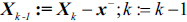
sbs.subsets_

 9 features, 8 features ==> .... ==>1 feature

sbs.indices_

 # indices_ is the final feature combination when number of features ==r, here k_features=1

feature_ar[list(sbs.subsets_[0])]

 

for subset_features in sbs.subsets_:
    print( feature_ar[ list(subset_features) ] )

 

sbs.scores_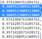

 

sbs.k_score_

 
plotting performance of feature subsets

# plotting performance of feature subsets
k_feat = [len(k) for k in sbs.subsets_] # len(k) is from X_train.shape[1] to k_features
 
plt.plot(k_feat, sbs.scores_, marker='o')
plt.ylim([0.7, 1.02])
plt.ylabel("Accuracy")
plt.xlabel("Number of features")
plt.grid()
plt.tight_layout()
plt.show()

 

 (total) 9 feature - 6 features = 3 : the index of bestFeaturesComb(when r=6)

sbs.subsets_[3]

 

x_train_df[ column_name_list ] ==> select columns 

x_train[feature_ar[ list(sbs.subsets_[3]) 
                  ]
       ]

# Tuning of K- value for Train & Test data

dummyarray = np.empty( (5,3) ) # 3 since ["K_value","Train_acc","Test_acc"]
k_valchart_df = pd.DataFrame( dummyarray ) #
k_valchart_df.columns = ["K_value","Train_acc","Test_acc"]

k_vals = [1,2,3,4,5, 6, 7, 8, 9, 10]

for i in range( len(k_vals) ):
    knn_fit = KNeighborsClassifier( n_neighbors=k_vals[i],
                                    p = 2,
                                    metric = 'minkowski'
                                  )
    x_train = x_train[ feature_ar[ list(sbs.subsets_[3]) ]
                     ]#######
    x_test = x_test[ feature_ar[ list(sbs.subsets_[3]) ]
                   ]  ######
                                               # 9-6=3
    knn_fit.fit( x_train, y_train )
    
    print( '\nK-value', k_vals[i] )
    
    tr_accuracy = round( accuracy_score( y_train, knn_fit.predict(x_train) ),
                         3
                       )
    print( '\nK-Nearest Neighbors - Train Confusion Matrix\n\n', 
           pd.crosstab( y_train, knn_fit.predict( x_train ),
                        rownames = ['Actuall'], colnames=['Predicted']
                      )
         )
    print( '\nK-Nearest Neighbors - Train accuracy:', tr_accuracy )
    print( '\nK-Nearest Neighbors - Train Classification Report\n', 
           classification_report( y_train, knn_fit.predict(x_train) )
         )
    
    ts_accuracy = round( accuracy_score( y_test, knn_fit.predict(x_test) ),
                         3
                       )
    print( '\nK-Nearest Neighbors - Test Confusion Matrix\n\n', 
           pd.crosstab( y_test, knn_fit.predict( x_test ),
                        rownames = ['Actuall'], colnames=['Predicted']
                      )
         )
    print( '\nK-Nearest Neighbors - Test accuracy:', ts_accuracy )
    print( '\nK-Nearest Neighbors - Test Classification Report\n', 
           classification_report( y_test, knn_fit.predict(x_test) )
         )
    
    k_valchart_df.loc[i, 'K_value'] = k_vals[i]
    k_valchart_df.loc[i, 'Train_acc'] = tr_accuracy
    k_valchart_df.loc[i, 'Test_acc'] = ts_accuracy

 ... ...

 ... ...

# Ploting accuracies over varied K-values
import matplotlib.pyplot as plt

plt.figure( figsize=(10,6) )
plt.xlabel( 'K-value' )
plt.ylabel( 'Accuracy' )
plt.plot( k_valchart_df['K_value'], k_valchart_df['Train_acc'], label='Train_acc', c='k' )
plt.plot( k_valchart_df['K_value'], k_valchart_df['Test_acc'], label='Test_acc', c='b')

plt.axis( [0.9, 10.5,
           0.92, 1.005
          ]
        )
plt.xticks( [1,2,3,4,5, 6, 7, 8, 9, 10] )

for a,b in zip( k_valchart_df['K_value'], k_valchart_df['Train_acc'] ):
    plt.text( a,b, str(b), fontsize=10, c='k' )

for a,b in zip( k_valchart_df['K_value'], k_valchart_df['Test_acc'] ):
    plt.text( a,b, str(b), fontsize=10, c='b' )

plt.legend( loc='upper right' )
plt.show()

from sklearn.neighbors import KNeighborsClassifier

x_train = x_train[ feature_ar[ list(sbs.subsets_[3]) ]
                 ]#######
x_test = x_test[ feature_ar[ list(sbs.subsets_[3]) ]
               ]  ######

knn_fit = KNeighborsClassifier( n_neighbors=3, p=2, 
                                metric='minkowski'
                              )
knn_fit.fit( x_train, y_train )

print( '\nK-Nearest Neighbors - Test Confusion Matrix\n\n', 
       pd.crosstab( y_test, knn_fit.predict(x_test),
                    rownames=['Actuall'], colnames=['Predicted']
                  )
     )
print( '\nK-Nearest Neighbors - Test Accuracy: ',
       round( accuracy_score(y_test, knn_fit.predict(x_test) ),
              3
            )
     )
print( '\nK-Nearest Neightbors-Test Classification Report\n',
       classification_report( y_test, knn_fit.predict(x_test) )
     )

it is appearing that KNN is working better now in classifying malignant and benign classes, obtaining test accuracy of 98.1 percent with 97 percent of recall on malignant class.

from sklearn.model_selection import train_test_split

x_vars_stdscale_df = pd.DataFrame( x_vars_stdscale, 
                                   index = x_vars.index,
                                   columns = x_vars.columns
                                 )
x_train, x_test, y_train, y_test = train_test_split( x_vars_stdscale_df,
                                                     y_var,
                                                     train_size=0.7,
                                                     random_state=42
                                                   )
x_train

Naive Bayes

     Bayes algorithm concept is quite old and exists from the 18th century. Thomas Bayes developed the foundational mathematical principles for determining the probability of unknown events from the known events. For example, if all apples are red in color and average diameter would be about 4 inches then, if at random one fruit is selected from the basket with red color and diameter of 3.7 inches, what is the probability that the particular fruit would be an apple? Naive term does assume independence of particular features in a class with respect to others. In this case, there would be no dependency between color and diameter. This independence assumption makes the Naive Bayes classifier most effective in terms of computational ease for particular tasks such as email classification based on words in which high dimensions of vocab do exist, even after assuming independence between features. Naive Bayes classifier performs surprisingly really well in practical applications.

     Bayesian classifiers are best applied to problems in which information from a very high number of attributes should be considered simultaneously to estimate the probability of final outcome. Bayesian methods utilize all available evidence to consider for prediction even features have weak effects on the final outcome to predict. However, we should not ignore the fact that a large number of features with relatively minor effects, taken together its combined impact would form strong classifiers.

Probability fundamentals

     Before diving into Naive Bayes, it would be good to reiterate the fundamentals. Probability of an event can be estimated from observed data by dividing the number of trails in which an event occurred with the total number of trails. For instance, if a bag contains red and blue balls and randomly picked 10 balls one by one with replacement and out of 10, 3 red balls appeared in trails we can say that probability of red is 0.3, = 3/10 = 0.3. Total probability of all possible outcomes must be 100 percent.

     If a trail has two outcomes such as email classification either it is spam or ham垃圾信息或正常信息 and both cannot occur simultaneously, these events are considered as mutually exclusive with each other. In addition, if those outcomes cover all possible events, it would be called as exhaustive events相互排斥事件. For example, in email classification if P (spam) = 0.1, we will be able to calculate P (ham) = 1- 0.1 = 0.9, these two events are mutually exclusive. In the following Venn diagram, all the email possible classes are represented (the entire universe) with the type of outcomes:

Joint probability

     Though mutually exclusive cases are simple to work upon, most of the actual problems do fall under the category of non-mutually exclusive events非互斥事件. By using the joint appearance, we can predict the event outcome. For example, if emails messages present the word like lottery, which is very highly likely of being spam rather than ham. The following Venn diagram indicates the joint probability of spam with lottery. However, if you notice in detail, lottery circle is not contained completely within the spam circle. This implies that not all spam messages contain the word lottery and not every email with the word lottery is spam.

     In the following diagram, we have expanded the spam and ham category in addition to the lottery word in Venn diagram representation:

     We have seen that 10 percent of all the emails are spam and 4 percent of emails have the word lottery and our task is to quantify the degree of overlap between these two proportions. In other words, we need to identify the joint probability of both p(spam) and p(lottery) occurring, which can be written as p(spam ∩ lottery). In case if both the events are totally unrelated, they are called independent events and their respective value is p(spam ∩ lottery) = p(spam) * p(lottery) = 0.1 * 0.04 = 0.004, which is 0.4 percent of all messages are spam containing the word Lottery. In general, for independent events P(A∩ B) = P(A) * P(B).

Understanding Bayes theorem with conditional probability

     Conditional probability provides a way of calculating relationships between dependent events using Bayes theorem. For example, A and B are two events and we would like to calculate P(A\B) can be read as the probability of an event occurring A given the fact that event B already occurred, in fact, this is known as conditional probability, the equation can be written as follows:

     To understand better, we will now talk about the email classification example. Our objective is to predict whether an email is a spam given the word lottery and some other clues. In this case, we already knew the overall probability of spam, which is 10 percent also known as prior probability. Now suppose you have obtained an additional piece of information that probability of word lottery in all messages, which is 4 percent, also known as marginal likelihood. Now, we know the probability that lottery was used in previous spam messages and is called the likelihood.

      By applying the Bayes theorem to the evidence, we can calculate the posterior probability that calculates the probability that the message is how likely a spam; given the fact that lottery was appearing in the message. On average if the probability is greater than 50 percent it indicates that the message is spam rather than ham.

     In the previous table, the sample frequency table that records the number of times Lottery
appeared in spam and ham messages and its respective likelihood has been shown. Likelihood table reveals that P(Lottery\Spam)= 3/22 = 0.13, indicating that probability is 13 percent that a spam message contains the term Lottery. Subsequently we can calculate the P(Spam ∩ Lottery) = P(Lottery\Spam) * P(Spam) = (3/22) * (22/100) = 0.03. In order to calculate the posterior probability, we divide P(Spam ∩ Lottery) with P(Lottery), which means (3/22)*(22/100) / (4/100) = 0.75. Therefore, the probability is 75 percent that a message is spam, given that message contains the word Lottery. Hence, don't believe in quick fortune guys!

Naive Bayes classification

     In the past example, we have seen with a single word called lottery, however, in this case, we will be discussing with a few more additional words such as Million(W2) and Unsubscribe(W3) to show how actual classifiers do work. Let us construct the likelihood table for the appearance of the three words (W1, W2, and W3), as shown in the following table for 100 emails:

     When a new message is received, the posterior probability will be calculated to determine that email message is spam or ham. Let us assume that we have an email with terms Lottery and Unsubscribe, but it does not have word Million in it, with this details, what is the probability of spam?

     By using Bayes theorem, we can define the problem as Lottery = Yes, Million = No and Unsubscribe = Yes:

     Solving the preceding equations will have high computational complexity due to the dependency of words with each other. As a number of words are added, this will even explode and also huge memory will be needed for processing all possible intersecting events. This finally leads to intuitive turnaround with independence of words (crossconditional independence) for which it got name of the Naive prefix for Bayes classifier. When both events are independent we can write P(A ∩ B) = P(A) * P(B). In fact, this equivalence is much easier to compute with less memory requirement:

In a similar way, we will calculate the probability for ham messages as well, as follows:

     By substituting the preceding likelihood table in the equations, due to the ratio of spam/ham we can just simply ignore the denominator terms in both the equations. Overall likelihood of spam is:

      After calculating the ratio, 0.008864/0.004349 = 2.03, which means that this message is two times more likely to be spam than ham这意味着该邮件是垃圾邮件的可能性是正常的两倍. But we can calculate the probabilities as follows:

     By converting likelihood values into probabilities, we can show in a presentable way for either to set-off some thresholds, and so on.

Laplace estimator

     In the previous calculation, all the values are nonzeros, which makes calculations well. Whereas in practice some words never appear in past for specific category and suddenly appear at later stages, which makes entire calculations as zeros.

     For example, in the previous equation W3(Unsubscribe) did have a 0 value instead of 13, and it will convert entire equations to 0 altogether:

     In order to avoid this situation, Laplace estimator essentially adds a small number to each of the counts in the frequency table, which ensures that each feature has a nonzero probability of occurring with each class. Usually, Laplace estimator is set to 1, which ensures that each class-feature combination is found in the data at least once:
Here is approximately equal to 0

     If you observe the equation carefully, value 1 is added to all three words in the numerator and at the same time, three has been added to all denominators to provide equivalence.

Naive Bayes SMS spam classification example

     Naive Bayes classifier has been developed using the SMS spam collection data available at
SMS Spam Collection. In this chapter, various techniques available in NLP techniques have been discussed to preprocess prior to build the Naive Bayes model:
UCI Machine Learning Repository: SMS Spam Collection Data Set
Index of /ml/machine-learning-databases/00228

import csv
import requests

url = 'https://archive.ics.uci.edu/ml/machine-learning-databases/00228/smsspamcollection.zip'
r = requests.get(url)

with open ('smsspamcollection.zip', 'wb') as f:
    f.write( r.content )

 ​

import zipfile
zip_file = zipfile.ZipFile('./smsspamcollection.zip')
zip_list = zip_file.namelist()

zip_list

 ​

for f in zip_list:
    zip_file.extract( f )
zip_file.close()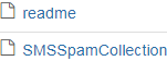

 ​

smsdata = open('SMSSpamCollection','r')
csv_reader = csv.reader(smsdata, delimiter='\t')
csv_reader

 ​

Normal coding starts from here as usual:

smsdata_data = []
smsdata_labels = []

for line in csv_reader:
    smsdata_labels.append(line[0])
    smsdata_data.append(line[1])
    
smsdata.close()

 The following code prints the top 5 lines:

for i in range(5):
    print( smsdata_data[i] )
    print( smsdata_labels[i])

​

 After getting preceding output run following code:

from collections import Counter

c = Counter( smsdata_labels )
print(c)

​  # 4825 + 747 = 5572

     Out of 5,572 observations, 4,825 are ham messages, which are about 86.5 percent and 747
spam messages are about remaining 13.4 percent.

     Using NLP techniques, we have preprocessed the data for obtaining finalized word vectors
to map with final outcomes spam or ham. Major preprocessing stages involved are: 

• Removal of punctuations:
       Punctuations needs to be removed before applying any further processing. Punctuations from the string library are !"#$%&\'()*+,-./:;<=>?@[\\]^_`{|}~, which are removed from all the messages.16_NLP stateful CharRNN_window_Tokenizer_stationary_colab_ResetState_character word level_regex_IMDb_Linli522362242的专栏-CSDN博客

  tf.keras.preprocessing.text.Tokenizer(
      num_words=None,
      filters='!"#$%&()*+,-./:;<=>?@[\\]^_`{|}~\t\n',
      lower=True, split=' ', char_level=False, oov_token=None,
      document_count=0, **kwargs
  )

  OR

  import re
   
  def preprocessor(text):
      text = re.sub( '<[^>]*>', '', 
                     text) #remove html tag: <a>, <br />
      print(text)
      emoticons = re.findall( '(?::|;|=)(?:-)?(?:\)|\(|D|P)', 
                             text)
      print(emoticons)
      # ' '.join(emoticons) is not empty then .replace('-', '')
      print(' '.join(emoticons).replace('-', ''))
      text = ( re.sub( '[\W]+', ' ', # [\W]+ == [^A-Za-z0-9_]+ # [^A-Za-z0-9_] : '(' or ')' or ':'
                       text.lower() # replace any [^A-Za-z0-9_] with ' '
                     ) +
               ' '.join(emoticons).replace('-', '') # put the emoticons at the end
             )
      return text
   
  preprocessor('is seven.<br /><br />Title (Brazil): Not Available')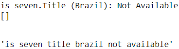

  

  preprocessor( "</a>This :) is :( a test : -)!" )

  

• Word tokenization:
  Words are chunked from sentences based on white space for further processing.

  def tokenizer(text):
      return text.split()
   
  tokenizer('runners like running and thus they run')

  
  OR

  tf.keras.preprocessing.text.Tokenizer(
      num_words=None,
      filters='!"#$%&()*+,-./:;<=>?@[\\]^_`{|}~\t\n',
      lower=True, split=' ', char_level=False, oov_token=None,
      document_count=0, **kwargs
  )

  num_words	the maximum number of words to keep, based on word frequency. Only the most common num_words-1 words will be kept.
  filters	a string where each element is a character that will be filtered from the texts. The default is all punctuation, plus tabs and line breaks, minus the ' character.
  lower	boolean. Whether to convert the texts to lowercase.
  split	str. Separator for word splitting.
  char_level	if True, every character will be treated as a token.
  oov_token	if given, it will be added to word_index and used to replace out-of-vocabulary words during text_to_sequence calls

  https://www.tensorflow.org/api_docs/python/tf/keras/preprocessing/text/Tokenizer
• Converting words into lowercase:
       Converting to all lower case provides removal of duplicates, such as Run and run, where the first one comes at start of the sentence and the later one comes in the middle of the sentence, and so on, which all needs to be unified to remove duplicates as we are working on bag of words technique.
• Stop word removal:
       Stop words are the words that repeat so many times in literature and yet are not a differentiator in the explanatory power of sentences.
  
       Stop-words are simply those words that are extremely common in all sorts of texts and probably bear no (or only a little) useful information that can be used to distinguish between different classes of documents. Examples of stopwords are is, and, has, and so on. Removing stop-words can be useful if we are working with raw or normalized term frequencies rather than tf-idfs(可以用于减轻特征向量中这些频繁出现的单词的权重。), which are already downweighting frequently occurring words.
  
  For example: I, me, you, this, that, and so on, which needs to be removed before
  further processing.

  import nltk
   
  nltk.download('stopwords')
  
  
  from nltk.corpus import stopwords
   
  stop = stopwords.words('english')
  [ w for w in tokenizer_porter('a runner likes running and runs a lot')
    if w not in stop]

  Stop word removal<==Stemming of words<== original text('a runner likes running and runs a lot')
• of length at least three:
  Here we have removed words with length less than three.
• Stemming of words:
       Stemming process stems the words to its respective root words. Example of stemming is bringing down running to run or runs to run. By doing stemming we reduce duplicates and improve the accuracy of the model.

  
  from nltk.stem.porter import PorterStemmer
   
  porter = PorterStemmer()
   
  def tokenizer_porter(text):
      return [porter.stem(word) for word in text.split()]
   
  tokenizer_porter('runners like running and thus they run')

  
       Using the PorterStemmer from the nltk package, we modified our tokenizer function to reduce words to their root form, which was illustrated by the simple preceding example where the word 'running' was stemmed to its root form 'run'.

• Part-of-speech (POS) tagging词性 (POS) 标记:
       This applies the speech tags to words, such as noun, verb, adjective, and so on.
  
       For example, POS tagging for running is verb, whereas for run is noun. In some situation running is noun and lemmatization will not bring down the word to root word run, instead, it just keeps the running as it is. Hence, POS tagging is a very crucial step necessary for performing prior to applying the lemmatization operation to bring down the word to its root word.
• Lemmatization of words:
       Lemmatization词形还原 is another different process to reduce
  the dimensionality. In lemmatization process, it brings down the word to root word rather than just truncating the words. For example, bring ate to its root word as eat when we pass the ate word into lemmatizer with the POS tag as verb.
        in practice, it has been observed that stemming and lemmatization have little impact on the performance of text classification (Influence of Word Normalization on Text Classification, Michal Toman, Roman Tesar, and Karel Jezek, Proceedings of InSciT, pages 354–358, 2006)

     The nltk package has been utilized for all the preprocessing steps, as it consists of all the necessary NLP functionality in one single roof:

import nltk
nltk.download('punkt')
nltk.download('averaged_perceptron_tagger')
nltk.download('wordnet')

from nltk.corpus import stopwords
from nltk.stem import WordNetLemmatizer
import string
import pandas as pd
from nltk import pos_tag
from nltk.stem import PorterStemmer

     Function has been written (preprocessing) consists of all the steps for convenience. However, we will be explaining all the steps in each section:

def preprocessing( text ):
    print(text)

Go until jurong point, crazy.. Available only in bugis n great world la e buffet... Cine there got amore wat...

• step 1. The following line of the code splits the word and checks each character if it is in standard punctuations if so it will be replaced with blank and or else it just does not replace with blanks:
   

  string.punctuation

  String of ASCII characters which are considered punctuation characters in the C locale: !"#$%&'()*+,-./:;<=>?@[\]^_`{|}~

      text2 = " ".join( "".join( [" " if ch in string.punctuation else ch # Removal of punctuations
                                      for ch in text
                                 ]
                               ).split()
                      )
      print(text2)

  Go until jurong point crazy Available only in bugis n great world la e buffet Cine there got amore wat

• step 2. The following code tokenizes the sentences into words based on white spaces and put them together as a list for applying further steps:
  nltk.tokenize package — NLTK 3.6.2 documentation
  
  nltk.tokenize.sent_tokenize(text, language='english')
       Return a sentence-tokenized copy of text, using NLTK’s recommended sentence tokenizer (currently PunktSentenceTokenizer for the specified language).
  Parameters
  text – text to split into sentences
  language – the model name in the Punkt corpus
  
  nltk.tokenize.word_tokenize(text, language='english', preserve_line=False)
  Return a tokenized copy of text, using NLTK’s recommended word tokenizer (currently an improved TreebankWordTokenizer along with PunktSentenceTokenizer for the specified language).
  Parameters
  text (str) – text to split into words
  language – the model name in the Punkt corpus
  preserve_line (bool) – An option to keep the preserve the sentence and not sentence tokenize it.

      tokens = [ word for sent in nltk.sent_tokenize(text2)   # step2 Return a sentence-tokenized copy of text
                          for word in nltk.word_tokenize(sent)# Return a tokenized copy of text
               ]
      print(tokens)

  ['Go', 'until', 'jurong', 'point', 'crazy', 'Available', 'only', 'in', 'bugis', 'n', 'great', 'world', 'la', 'e', 'buffet', 'Cine', 'there', 'got', 'amore', 'wat']
  Note: The text here is only one paragraph so I can't see any effect, just word tokenize
• step 3. Converting all the cases (upper, lower, and proper) into lowercase reduces duplicates in corpus:

      tokens = [ word.lower() for word in tokens ]         # step3 Converting words into lowercase
      print( tokens )

  ['go','until', 'jurong', 'point', 'crazy', 'available', 'only', 'in', 'bugis', 'n', 'great', 'world', 'la', 'e', 'buffet', 'cine', 'there', 'got', 'amore', 'wat']
• step 4. As mentioned earlier, stop words are the words that do not carry much weight in understanding the sentence; they are used for connecting words, and so on. We have removed them with the following line of code:

      stopwds = stopwords.words('english')
      tokens = [token for token in tokens
                          if token not in stopwds          # step4 Stop word removal
               ]
      print( tokens )

  ['go', 'jurong', 'point', 'crazy', 'available', 'bugis', 'n', 'great', 'world', 'la', 'e', 'buffet', 'cine', 'got', 'amore', 'wat']
• step 5.Keeping only the words with length greater than 3 in the following code for removing small words, which hardly consists of much of a meaning to carry:

      tokens = [ word for word in tokens if len(word)>=3 ] # step5 of length at least three
      print( tokens )

  ['jurong', 'point', 'crazy', 'available', 'bugis', 'great', 'world', 'buffet', 'cine', 'got', 'amore', 'wat']
• step 6.Stemming is applied on the words using PorterStemmer function, which stems the extra suffixes[ˈsʌfɪksɪz from the words该函数从单词中提取额外的后缀(Stemming of words):

      stemmer = PorterStemmer()
      tokens = [ stemmer.stem(word) for word in tokens ]   # step 6 Stemming of words
      print( tokens )

  ['jurong', 'point', 'crazi', 'avail', 'bugi', 'great', 'world', 'buffet', 'cine', 'got', 'amor', 'wat']
• step 7.POS tagging is a prerequisite for lemmatization, based on whether the word is noun or verb, and so on, it will reduce it to the root word:

      tagged_corpus = pos_tag( tokens )                    # step 7 POS tagging
      print( tagged_corpus )    # e.g. [('They', 'PRP'), ('refuse', 'NN'), ...]

  [('jurong', 'JJ'), ('point', 'NN'), ('crazi', 'NN'), ('avail', 'NN'), ('bugi', 'NN'), ('great', 'JJ'), ('world', 'NN'), ('buffet', 'NN'), ('cine', 'NN'), ('got', 'VBD'), ('amor', 'JJ'), ('wat', 'NN')]
  
  https://www.nltk.org/book/ch05.html
  A part-of-speech tagger, or POS-tagger, processes a sequence of words, and attaches a part of speech tag to each word (don't forget to import nltk)词性标注器或词性标注器处理一系列单词，并为每个单词附加一个词性标签（不要忘记导入 nltk）：

  text = word_tokenize("And now for something completely different")
  nltk.pos_tag(text)

  ​Here we see that
  And is CC, a coordinating conjunction;
  now and completely are RB, or adverbs副词;
  for is IN, a preposition介词;
  something is NN, a noun; and
  different is JJ, an adjective.
  
  Let's look at another example, this time including some homonyms[ˈhɑːmənɪm,ˈhoʊmənɪm]同音异义词:

  text = word_tokenize("They refuse to permit us to obtain the refuse permit")
  nltk.pos_tag(text)

  ​
       Notice that refuse and permit both appear as a present tense verb (VBP) 动词现在时and a noun (NN). E.g. refuse is a verb meaning "deny," while REFuse is a noun meaning "trash" (i.e. they are not homophones). Thus, we need to know which word is being used in order to pronounce the text correctly. (For this reason, text-to-speech systems usually perform POS-tagging.)
  
  
       Observe that searching for woman finds nouns; searching for bought mostly finds verbs; searching for over generally finds prepositions; searching for the finds several determiners. A tagger can correctly identify the tags on these words in the context of a sentence, e.g. The woman bought over $150,000 worth of clothes.
  
       A tagger can also model our knowledge of unknown words标注器还可以对我们对未知单词的知识进行建模, e.g. we can guess that scrobbling is probably a verb, with the root scrobble, and likely to occur in contexts like he was scrobbling.

• step 8.The pos_tag function returns the part of speed in four formats for noun and six formats for verb.
  NN (noun, common, singular), NNP (noun, proper, singular), NNPS (noun, proper专有, plural), NNS (noun, common, plural),
  VB (verb, base form), VBD (verb, past tense), VBG (verb, present participle现在分词), VBN (verb, past participle), VBP (verb, present tense, not third person singular非第三人称单数), VBZ (verb, present tense, third person singular):

      Noun_tags = ['NN','NNP','NNPS','NNS']
      Verb_tags = ['VB','VBD','VBG','VBN','VBP','VBZ']

Previous complete codeLemmatization Approaches with Examples in Python

def preprocessing( text ):
    #print(text)
    
    text2 = " ".join( "".join( [" " if ch in string.punctuation else ch # Removal of punctuations
                                    for ch in text
                               ]
                             ).split()
                    )
    #print(text2)
    
    tokens = [ word for sent in nltk.sent_tokenize(text2)   # step2 Return a sentence-tokenized copy of text
                        for word in nltk.word_tokenize(sent)# Return a tokenized copy of text
             ]
    #print(tokens)
    
    tokens = [ word.lower() for word in tokens ]         # step3 Converting words into lowercase
    #print( tokens )
    
    stopwds = stopwords.words('english')
    tokens = [token for token in tokens
                        if token not in stopwds          # step4 Stop word removal
             ]
    #print( tokens )
    
    tokens = [ word for word in tokens if len(word)>=3 ] # step5 of length at least three
    #print( tokens )
    
    stemmer = PorterStemmer()
    tokens = [ stemmer.stem(word) for word in tokens ]   # step 6 Stemming of words
    #print( tokens )
    
    tagged_corpus = pos_tag( tokens )                    # step 7 POS tagging
    #print( tagged_corpus )    # e.g. [('They', 'PRP'), ('refuse', 'NN'), ...]
    
    Noun_tags = ['NN','NNP','NNPS','NNS']
    Verb_tags = ['VB','VBD','VBG','VBN','VBP','VBZ']
    
    lemmatizer = WordNetLemmatizer()                    # step8, 9Lemmatization of words
    
    def prat_lemmatize( token, tag ):
        if tag in Noun_tags:
            return lemmatizer.lemmatize( token, 'n' )
        elif tag in Verb_tags:
            return lemmatizer.lemmatize( token, 'v' )
        else:
            return lemmatizer.lemmatize( token, 'n' )
    ####
    pre_proc_text = " ".join( [ prat_lemmatize(token, tag) for token,tag in tagged_corpus
                                  ] )
    #print(pre_proc_text)
    return pre_proc_text

     The following step applies the preprocessing function to the data and generates new corpus:

smsdata_data_2 = []
for i in smsdata_data:
    smsdata_data_2.append( preprocessing(i) )
smsdata_data_2

     Data will be split into train and test based on 70-30 split and converted to the NumPy array for applying machine learning algorithms:

import numpy as np

trainset_size = int( round( len(smsdata_data_2)*0.70 ) )
print( 'The training set size for this classifier is ' +\
       str( trainset_size ) + '\n'
     )

x_train = np.array( [ ''.join(rec)
                      for rec in smsdata_data_2[0:trainset_size] 
                    ]
                  )
y_train = np.array( [ rec 
                      for rec in smsdata_labels[0:trainset_size]
                    ]
                  )
x_test = np.array( [ ''.join(rec)
                      for rec in smsdata_data_2[ trainset_size: len(smsdata_data_2) ] 
                   ]
                 )
y_test = np.array( [ rec 
                      for rec in smsdata_labels[ trainset_size: len(smsdata_data_2) ]
                    ]
                  )
len(x_train), len(y_train), len(x_test), len(y_test)

    The following code converts the words into a vectorizer format and applies term frequency-inverse document frequency (TF-IDF) weights, which is a way to increase weights to words with high frequency and at the same time penalize the general terms such as the, him, at, and so on. In the following code, we have restricted to most frequent 4,000 words in the vocabulary, none the less we can tune this parameter as well for checking where the better accuracies are obtained:

tf-idfs in scikitlearn

cp8_Sentiment_urlretrieve_pyprind_tarfile_bag词袋_walk目录_regex_verbose_N-gram_Hash_colab_verbose_文本向量化_Linli522362242的专栏-CSDN博客

     However, if we'd manually calculated the tf-idfs of the individual terms in our feature vectors, we would have noticed that TfidfTransformer calculates the tf-idfs slightly differently compared to the standard textbook equations( and ). The equation for the inverse document frequency implemented in scikitlearn is computed as follows:
 ,     is the total number of documents, and df(d, t) is the number of documents, d, that contain the term t.

     Similarly, the tf-idf (term frequency-inverse document frequency) computed in scikit-learn deviates偏离 slightly from the default equation we defined earlier:

tf(t, d) is the term frequency(the number of times a term, t, occurs in a document, d.)

     Note that the "+1" in the previous equations is due to setting smooth_idf=True in the previous code example(), which is helpful for assigning zero-weight (that is,
idf(t, d) = log(1) = 0) to terms that occur in all documents.

     While it is also more typical to normalize the raw term frequencies before calculating the tf-idfs, the TfidfTransformer class normalizes the tf-idfs directly. By default
(norm='l2'), scikit-learn's TfidfTransformer applies the L2-normalization, which returns a vector of length 1 by dividing an unnormalized feature vector, v, by its L2-norm: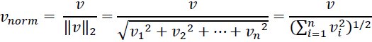

    To make sure that we understand how TfidfTransformer works, let's walk through an example and calculate the tf-idf of the word 'is' in the third document. The document frequency of this term is 3 since the term 'is' occurs in all three documents (df = 3). Thus, we can calculate the inverse document frequency as follows:
  <== <== =3
     Now, in order to calculate the tf-idf, we simply need to add 1 to the inverse document frequency and multiply it by the term frequency:
   The word 'is' has a term frequency of 3 (tf = 3) in the third document

     If we repeated this calculation for all terms in the third document, we'd obtain the following tf-idf vectors: [3.39, 3.0, 3.39, 1.29, 1.29, 1.29, 2.0, 1.69, 1.29]. However, notice that the values in this feature vector are different from the values that we obtained from TfidfTransformer that we used previously. The final step that we are missing in this tf-idf calculation is the L2-normalization, which can be applied as follows: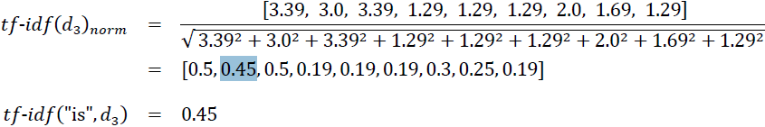

sklearn.feature_extraction.text.TfidfVectorizer — scikit-learn 0.24.2 documentation

• min_df        float or int, default=1
  
                      When building the vocabulary ignore terms that have a document frequency strictly lower than the given threshold. This value is also called cut-off in the literature.
  
  If float in range of [0.0, 1.0], the parameter represents a proportion of documents, integer absolute counts. This parameter is ignored if vocabulary is not None.

• ngram_range : tuple (min_n, max_n), default=(1, 1)

                            The lower and upper boundary of the range of n-values for different n-grams to be extracted. All values of n such that min_n <= n <= max_n will be used. For example an ngram_range of (1, 1) means only unigrams单元组(1-gram: "the", "sun", "is", "shining"), (1, 2) means unigrams and bigrams二元组(2-gram: "the sun", "sun is", "is shining"), and (2, 2) means only bigrams. Only applies

• stop_words : {‘english’}, list, default=None
                         If a string, it is passed to _check_stop_list and the appropriate stop list is returned. ‘english’ is currently the only supported string value. There are several known issues with ‘english’ and you should consider an alternative (see Using stop words, stop words : probably bear no (or only a little) useful information that can be used to distinguish between different classes of documents, Examples of stopwords are is, and, has, and like).

                         If a list, that list is assumed to contain stop words, all of which will be removed from the resulting tokens. Only applies if analyzer == 'word'.

                         If None, no stop words will be used. max_df can be set to a value in the range [0.7, 1.0) to automatically detect and filter stop words based on intra corpus document frequency of terms.
   

• strip_accents : {‘ascii’, ‘unicode’}, default=None
                            Remove accents重音 and perform other character normalization during the preprocessing step. ‘ascii’ is a fast method that only works on characters that have an direct ASCII mapping. ‘unicode’ is a slightly slower method that works on any characters. None (default) does nothing.
                            Both ‘ascii’ and ‘unicode’ use NFKD normalization from unicodedata.normalize.

• analyzer ：{‘word’, ‘char’, ‘char_wb’} or callable, default=’word’

• norm{‘l1’, ‘l2’},  default=’l2’

  Each output row will have unit norm, either: * ‘l2’: Sum of squares of vector elements is 1. The cosine similarity between two vectors is their dot product when l2 norm has been applied. * ‘l1’: Sum of absolute values of vector elements is 1. See preprocessing.normalize.

• smooth_idf  bool, default=True

  Smooth idf weights by adding one to document frequencies, as if an extra document was seen containing every term in the collection exactly once. Prevents zero divisions.

# building TFIDF vectorizer
from sklearn.feature_extraction.text import TfidfVectorizer

vectorizer = TfidfVectorizer( min_df=2, ngram_range=(1,2), stop_words='english',
                              max_features=4000,
                              strip_accents='unicode',
                              norm='l2'
                            )

    The TF-IDF transformation has been shown as follows on both train and test data. The todense function is used to create the data to visualize the content:

x_train_2 = vectorizer.fit_transform( x_train ).todense()
x_test_2 = vectorizer.transform( x_test ).todense()

x_train_2

It can convert a matrix to an array as shown below.

np.asarray(x_train_2[0]).flatten()[490:500]

 

     Multinomial Naive Bayes classifier is suitable for classification with discrete features (example word counts), which normally requires large feature counts. However, in practice, fractional counts such as TF-IDF will also work well. If we do not mention any Laplace estimator, it does take the value of 1.0 means and it will add 1.0 against each term in numerator and total for denominator:

from sklearn.naive_bayes import MultinomialNB  # Multinomial Naive Bayes classifier

clf = MultinomialNB().fit( x_train_2, y_train )

ytrain_nb_predicted = clf.predict( x_train_2 )
ytest_nb_predicted = clf.predict( x_test_2 )

from sklearn.metrics import classification_report, accuracy_score

print( '\nNaive Bayes - Train Confusion Matrix\n\n',
       pd.crosstab( y_train, ytrain_nb_predicted,
                    rownames=['Actuall'], colnames=['Predicted']
                  )
     )
print( '\nNaive Bayes - Train Accuracy',
       round( accuracy_score(y_train, ytrain_nb_predicted),
              3
            )
     )
print( '\nNaive Bayes - Train Classification Report\n',
       classification_report( y_train, ytrain_nb_predicted )
     )
#####
print( '\nNaive Bayes - Test Confusion Matrix\n\n',
       pd.crosstab( y_test, ytest_nb_predicted,
                    rownames=['Actuall'], colnames=['Predicted']
                  )
     )
print( '\nNaive Bayes - Test Accuracy',
       round( accuracy_score(y_test, ytest_nb_predicted),
              3
            )
     )
print( '\nNaive Bayes - Test Classification Report\n',
       classification_report( y_test, ytest_nb_predicted )
     )

From the previous results, it is appearing that Naive Bayes has produced excellent results of 96.3 percent test accuracy with significant recall value of 74 percent for spam and almost 100 percent for ham.

     However, if we would like to check what are the top 10 features based on their coefficients from Naive Bayes, the following code will be handy for this:

# printing top features

# printing top features
feature_names = vectorizer.get_feature_names() # max_features=4000
coefs = clf.coef_

intercept = clf.intercept_
coefs_with_fns = sorted( zip(clf.coef_[0], feature_names), reverse=True )

print( '\n\nTop 10 features - both first & last\n' )
n=10
top_n_coefs = zip( coefs_with_fns[:n], coefs_with_fns[:-(n+1):-1] )
print('\tCoef\tFeature\t\t\tCoef\tFeature')
for (coef_top_10, featureName_top_10), (coef_last_10, featureName_last_10) in top_n_coefs:
    print( '\t%.4f\t%-15s\t\t%.4f\t%-15s' % (coef_top_10, featureName_top_10,
                                             coef_last_10, featureName_last_10
                                            )
         )

Summary

     In this chapter, you have learned about KNN and Naive Bayes techniques, which require somewhat a little less computational power. KNN, in fact, is called a lazy learner(it does not learn anything during the training phase like regression, random forest, and so on. Instead, it starts working only during the testing/evaluation phase to compare the given test observations with the nearest training observations, which will take significant time in comparing each test data point), as it does not learn anything apart from除了 comparing with training data points to classify them into class. Also, you have seen how to tune the k-value using grid search technique. Whereas explanation has been provided for Naive Bayes classifier, NLP examples have been provided with all the famous NLP processing techniques to give you a flavor of this field in a very crisp manner. Though in text processing, either Naive Bayes or SVM techniques could be used as these two techniques can handle data with high dimensionality, which is very relevant in NLP, as the number of word vectors is relatively high in dimensions and sparse at the same time.

     In the next chapter, we will be covering the details of unsupervised learning, more precisely, clustering and principal component analysis models.