cp8_Sentiment_urlretrieve_pyprind_tarfile_bag词袋_walk目录_regex_verbose_N-gram_Hash_colab_verbose_文本向量化

     In the modern internet and social media age, people's opinions, reviews, and recommendations have become a valuable resource for political science and businesses. Thanks to modern technologies, we are now able to collect and analyze such data most efficiently. In this chapter, we will delve into a subfield of natural language processing (NLP) called sentiment analysis and learn how to use machine learning algorithms to classify documents based on their polarity: the attitude of the writer. In particular, we are going to work with a dataset of 50,000 movie reviews from the Internet Movie Database (IMDb) and build a predictor that can distinguish between positive and negative reviews.

The topics that we will cover in the following sections include the following:

• • Cleaning and preparing text data
• • Building feature vectors from text documents
• • Training a machine learning model to classify positive and negative movie reviews
• • Working with large text datasets using out-of-core learning
• • Inferring topics from document collections for categorization

Preparing the IMDb movie review data for text processing

     As mentioned, sentiment[ˈsentɪmənt]情感 analysis, sometimes also called opinion mining, is a popular subdiscipline of the broader field of NLP; it is concerned with analyzing the polarity of documents. A popular task in sentiment analysis is the classification of documents based on the expressed opinions or emotions of the authors with regard to a particular topic.

     we will be working with a large dataset of movie reviews from the Internet Movie Database (IMDb) that has been collected by Andrew Maas and others. The movie review dataset consists of 50,000 polar movie reviews that are labeled as either positive or negative; here, positive means that a movie was rated with more than six stars on IMDb, and negative means that a movie was rated with fewer than five stars on IMDb. In the following sections, we will download the dataset, preprocess it into a useable format for machine learning tools, and extract meaningful information from a subset of these movie reviews to build a machine learning model that can predict whether a certain reviewer liked or disliked a movie.

(aclImdb_v1.tar.gz)Obtaining the movie review dataset

A compressed archive of the movie review dataset (84.1 MB) can be downloaded from Sentiment Analysis as a gzip-compressed tarball archive:

• • If you are working with Linux or macOS, you can open a new terminal window, cd into the download directory and execute tar -zxf aclImdb_v1.tar.gz to decompress the dataset.
• • If you are working with Windows, you can download a free archiver, such as 7-Zip (http://www.7-zip.org), to extract the files from the download archive.
• 
• Alternatively, you can directly unpack the gzip-compressed tarball archive directly in Python as follows:

# install selenium
# https://blog.csdn.net/Linli522362242/article/details/94811754
from selenium import webdriver

from lxml import etree

url = "http://ai.stanford.edu/~amaas/data/sentiment/"

driver = webdriver.Chrome(executable_path="C:/chromedriver/chromedriver")
driver.get('http://ai.stanford.edu/~amaas/data/sentiment/') 

pageSource = driver.page_source

selector = etree.HTML(pageSource)
targetFile_href=selector.xpath('//a[contains(text(), "Large Movie Review Dataset v1.0")]/@href')[0]

sourceUrl = url+targetFile_href # targetFile_href : 'aclImdb_v1.tar.gz'
# sourceUrl : 'http://ai.stanford.edu/~amaas/data/sentiment/aclImdb_v1.tar.gz'

import urllib.request
import time
import sys
import os

def reporthook(count, block_size, total_size):
    global start_time
    if count==0:
        start_time = time.time()
        return
    duration = time.time() - start_time
    progress_size = int(count*block_size)
    currentLoad = progress_size/(1024.**2)
    speed = currentLoad / duration # 1024.**2 <== 1MB=1024KB, 1KB=1024Btyes
    percent = count * block_size * 100./total_size
    sys.stdout.write("\r%d%% | %d MB | speed=%.2f MB/s | %d sec elapsed" %
                     (percent, currentLoad, speed, duration)
                    )
    sys.stdout.flush()

# if neither exists foler('aclImdb') nor file ('aclImdb_v1.tar.gz') then download...
if not os.path.isdir('aclImdb') and not os.path.isfile('aclImdb_v1.tar.gz'):
    # urllib.request.urlretrieve(url, filename=None, reporthook=None, data=None)
    # The third argument, if present, is a callable that will be called once on establishment of 
    # the network connection and once after each block read thereafter. 
    # The callable will be passed three arguments; a count of blocks transferred so far, 
    #                                              a block size in bytes, 
    #                                              and the total size of the file. (bytes)
    urllib.request.urlretrieve(sourceUrl, targetFile_href, reporthook)

os.path.isdir() method in Python is used to check whether the specified path is an existing directory or not

import tarfile

if not os.path.isdir(targetFile_href):
    with tarfile.open(targetFile_href, 'r:gz') as tar:
        tar.extractall()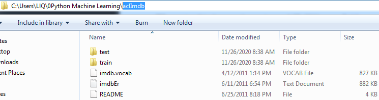

# os.getcwd() # OR # os.path.abspath('.') ==>'C:\\Users\\LlQ\\0Python Machine Learning'
for (root, dirs, files) in os.walk('aclImdb', topdown=True):
    print( root )
    print( dirs )
    print( files[:5] )
    print( '--------------------------------' )

 

from pathlib import Path

#Path(os.getcwd()) ==> Path(os.getcwd()) WindowsPath('C:/Users/LlQ/0Python Machine Learning')
path=Path(os.getcwd())/'aclImdb' 
path 

 

path.parts

 

for (currentDir, subdirs, files) in os.walk(path, topdown=True):
    indent = len( Path(currentDir).parts) - len(path.parts)
    # if len( Path(currentDir).parts) == len(path.parts) then indent=0; if not, indent>0 
    print("    " *indent + Path(currentDir).parts[-1] + os.sep)
    
    for index, filename in enumerate( sorted(files) ): #files is a list
        if index == 3:
            print("    " *(indent+1) + "...") #indent+1 since files
            break; #exist for loop
        print("    " *(indent+1) + filename)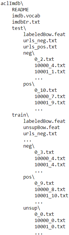

 13_Load Preproc4_[..., np.newaxis]_ExitStack_walk_file操作_timeit_regex_feature vector embed_Text Toke_Linli522362242的专栏-CSDN博客

Preprocessing the movie dataset into a more convenient format

     Having successfully extracted the dataset, we will now assemble the individual text documents from the decompressed download archive into a single CSV file. In the following code section, we will be reading the movie reviews into a pandas DataFrame object, which can take up to 10 minutes on a standard desktop computer. To visualize the progress and estimated time until completion, we will use the Python Progress Indicator (PyPrind, https://pypi.python.org/pypi/PyPrind/) package, which was developed several years ago for such purposes. PyPrind can be installed by executing the pip install pyprind command:

import pyprind
import pandas as pd

basepath = 'aclImdb'
labelDict = {'pos': 1, 'neg':0} # similar to labelEncoder
pbar = pyprind.ProgBar(50000) # initialization with number of iterations
df=pd.DataFrame()

for t in ('test', 'train'):
    for label in ('pos', 'neg'):
        path = os.path.join(basepath, t, label) # .../aclImdb/train/pos or .../aclImdb/train/neg  
        for file in sorted( os.listdir(path) ):#os.listdir(path)==>a list including files and folders
            with open(os.path.join(path, file), 'r', encoding='utf-8') as infile:
                txt = infile.read()
            df = df.append([ [txt, labelDict[label]] ], 
                            ignore_index=True)
            pbar.update() # ) update the progress visualization
df.columns=['review', 'sentiment']

print(df.head())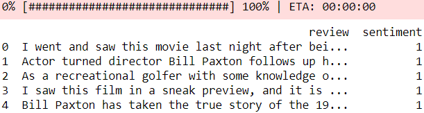

     In the preceding code, we first initialized a new progress bar object, pbar, with 50,000 iterations, which was the number of documents we were going to read in. Using the nested for loops, we iterated over the train and test subdirectories in the main aclImdb directory and read the individual text files from the pos and neg subdirectories that we eventually appended to the df pandas DataFrame, together with an integer class label (1 = positive and 0 = negative).

     Since the class labels in the assembled dataset are sorted, we will now shuffle DataFrame using the permutation function from the np.random submodule—this will be useful to split the dataset into training and test datasets in later sections, when we will stream the data from our local drive directly.

For our own convenience, we will also store the assembled and shuffled movie review dataset as a CSV file:

import numpy as np

np.random.seed(0)
df = df.reindex(np.random.permutation(df.index))
df.head()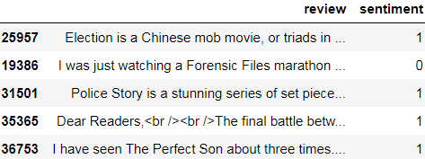

 <==

df.to_csv('movie_data.csv', index=False, encoding='utf-8')

     Since we are going to use this dataset later in this chapter, let's quickly confirm that we have successfully saved the data in the right format by reading in the CSV and
printing an excerpt of the first three examples:

df = pd.read_csv('movie_data.csv', encoding='utf-8')
df.head(3)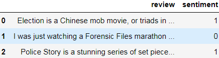

As a sanity check, before we proceed to the next section, let's make sure that the DataFrame contains all 50,000 rows:

df.shape

Introducing the bag-of-words model 

13_Load Preproc4_[..., np.newaxis]_ExitStack_walk_file操作_timeit_regex_feature vector embed_Text Toke_Linli522362242的专栏-CSDN博客

     You may remember from Cp4, Building Good Training Datasets – Data Preprocessing cp4 Training Sets Preprocessing_StringIO_dropna_categorical_feature_Encode_Scale_L1_L2_bbox_to_ancho_Linli522362242的专栏-CSDN博客, that we have to convert categorical data, such as text or words, into a numerical form before we can pass it on to a machine learning algorithm. In this section, we will introduce the bag-of-words model, which allows us to represent text as numerical feature vectors. The idea behind bag-of-words is quite simple and can be summarized as follows:

1. 1. We create a vocabulary of unique tokens—for example, words—from the entire set of documents.
2. 2. We construct a feature vector from each document that contains the counts of how often each word occurs in the particular document.

     Since the unique words in each document represent only a small subset of all the words in the bag-of-words vocabulary, the feature vectors will mostly consist of zeros, which is why we call them sparse. Do not worry if this sounds too abstract; in the following subsections, we will walk through the process of creating a simple bag-of-words model step by step.

Transforming words into feature vectors

     To construct a bag-of-words model based on the word counts in the respective documents, we can use the CountVectorizer class implemented in scikit-learn. As you will see in the following code section, CountVectorizer takes an array of text data, which can be documents or sentences, and constructs the bag-of-words model for us:

     By calling the fit_transform method on CountVectorizer, we just constructed the vocabulary of the bag-of-words model and transformed the following three sentences into sparse feature vectors:

1. The sun is shining
2. The weather is sweet
3. The sun is shining, the weather is sweet, and one and one is two

import numpy as np
from sklearn.feature_extraction.text import CountVectorizer

count = CountVectorizer()
docs = np.array([
    'The sun is shining',
    'The weather is sweet',
    'The sun is shining, the weather is sweet, and one and one is two'
])

bag = count.fit_transform(docs)

Now, let's print the contents of the vocabulary to get a better understanding of the underlying concepts: 

print( count.vocabulary_)

     As you can see from executing the preceding command, the vocabulary is stored in a Python dictionary that maps the unique words to integer indices. Next, let's print
the feature vectors that we just created:

print(bag.toarray())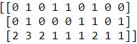

  # 3 ==> 1

     Each index position in the feature vectors shown here corresponds to the integer values that are stored as dictionary items in the CountVectorizer vocabulary. For
example, the first feature at index position 0 resembles the count of the word 'and', which only occurs in the last document, and the word 'is', at index position 1 (the
second feature in the document vectors), occurs in all three sentences. These values in the feature vectors are also called the raw term frequencies: tf(t, d)—the number
of times a term, t, occurs in a document, d. It should be noted that, in the bag-of-words model, the word or term order in a sentence or document does not matter. The order in which the term frequencies appear in the feature vector is derived from the vocabulary indices, which are usually assigned alphabetically.

N-gram models

     The sequence of items in the bag-of-words model that we just created is also called the 1-gram(1元组) or unigram(单元组) model—each item or token in the vocabulary represents a single word. More generally, the contiguous sequences of items in NLP(natural language processing)—words, letters, or symbols—are also called n-grams. The choice of the number, n, in the n-gram model depends on the particular application; for example, a study by Ioannis Kanaris and others revealed that n-grams of size 3 and 4 yield good performances in the anti-spam filtering of email messages (Words versus character n-grams for anti-spam filtering, Ioannis Kanaris, Konstantinos Kanaris, Ioannis Houvardas, and Efstathios Stamatatos, International Journal on Artificial Intelligence Tools, World Scientific Publishing Company, 16(06): 1047-1067, 2007).

     To summarize the concept of the n-gram representation, the 1-gram and 2-gram representations of our first document "the sun is shining" would be constructed as follows:

• • 1-gram: "the", "sun", "is", "shining"
• • 2-gram: "the sun", "sun is", "is shining"

The CountVectorizer class in scikit-learn allows us to use different n-gram models via its ngram_range parameter. While a 1-gram representation is used by default, we could switch to a 2-gram representation by initializing a new CountVectorizer instance with ngram_range=(2,2).

Assessing word relevancy via term frequency-inverse document frequency

     When we are analyzing text data, we often encounter words that occur across multiple documents from both classes. These frequently occurring words typically don't contain useful or discriminatory[dɪˈskrɪmɪnətɔri]歧视的,有辨识度的 information. In this subsection, you will learn about a useful technique called the term frequency-inverse document frequency (tf-idf), which can be used to downweight these frequently occurring words in the feature vectors. The tf-idf can be defined as the product of the term frequency and the inverse document frequency:

Here, tf(t, d) is the term frequency(the number of times a term, t, occurs in a document, d.) that we introduced in the previous section, and idf(t, d) is the inverse document frequency, which can be calculated as follows:

     Here, is the total number of documents, and df(d, t) is the number of documents, d, that contain the term t. Note that adding the constant 1 to the denominator is
optional and serves the purpose of assigning a non-zero value to terms that occur in none of the training examples; the log is used to ensure that low document frequencies are not given too much weight.

     The scikit-learn library implements yet another transformer, the TfidfTransformer class, which takes the raw term frequencies from the CountVectorizer class as input and transforms them into tf-idfs:

smooth_idf : bool, default=True  sklearn.feature_extraction.text.TfidfTransformer — scikit-learn 0.24.2 documentation

                      Smooth idf weights by adding one to document frequencies, as if an extra document was seen containing every term in the collection exactly once. Prevents zero divisions

from sklearn.feature_extraction.text import TfidfTransformer

tf_idf = TfidfTransformer(use_idf=True,
                          norm='l2',
                          smooth_idf=True)
print( tf_idf.fit_transform( count.fit_transform(docs) ) )

     Note that the "+1" in the previous equations is due to setting smooth_idf=True in the previous code example, which is helpful for assigning zero-weight (that is, idf(t, d) = log(1) = 0) to terms that occur in all documents. 

print( tf_idf.fit_transform( count.fit_transform(docs) ).toarray() )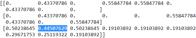

print( np.round(tf_idf.fit_transform( count.fit_transform(docs) ).toarray(),2) )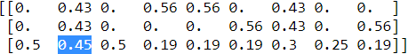

 # word:index

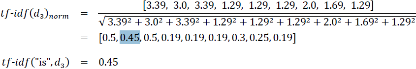
     As you saw in the previous subsection, the word 'is' had the largest term frequency in the third document, being the most frequently occurring word. However, after transforming the same feature vector into tf-idfs, the word 'is' is now associated with a relatively small tf-idf (0.45) in the third document, since it is also present in the first and second document and thus is unlikely to contain any useful discriminatory[dɪˈskrɪmɪnətɔri]歧视的,有辨识度的 information.

tf-idfs in scikitlearn

     However, if we'd manually calculated the tf-idfs of the individual terms in our feature vectors, we would have noticed that TfidfTransformer calculates the tf-idfs slightly differently compared to the standard textbook equations that we defined previously. The equation for the inverse document frequency implemented in scikitlearn is computed as follows:
       is the total number of documents, and df(d, t) is the number of documents, d, that contain the term t

Similarly, the tf-idf (term frequency-inverse document frequency) computed in scikit-learn deviates偏离 slightly from the default equation we defined earlier:

tf(t, d) is the term frequency(the number of times a term, t, occurs in a document, d.)

     Note that the "+1" in the previous equations is due to setting smooth_idf=True in the previous code example(), which is helpful for assigning zero-weight (that is,
idf(t, d) = log(1) = 0) to terms that occur in all documents.

     While it is also more typical to normalize the raw term frequencies before calculating the tf-idfs, the TfidfTransformer class normalizes the tf-idfs directly. By default
(norm='l2'), scikit-learn's TfidfTransformer applies the L2-normalization, which returns a vector of length 1 by dividing an unnormalized feature vector, v, by its L2-norm: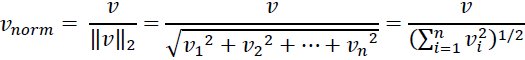

     To make sure that we understand how TfidfTransformer works, let's walk through an example and calculate the tf-idf of the word 'is' in the third document. The document frequency of this term is 3 since the term 'is' occurs in all three documents (df = 3). Thus, we can calculate the inverse document frequency as follows:
  <== 

Now, in order to calculate the tf-idf, we simply need to add 1 to the inverse document frequency and multiply it by the term frequency:

   The word 'is' has a term frequency of 3 (tf = 3) in the third document

tf_is = 3 # (the number of times a term, t, occurs in a document, d.)
n_d = 3
idf_is = np.log( (n_d+1)/(3+1) )
tfidf_is = tf_is * (idf_is+1)
print('tf-idf of term "is" = %.2f' % tfidf_is)

  

     If we repeated this calculation for all terms in the third document, we'd obtain the following tf-idf vectors: [3.39, 3.0, 3.39, 1.29, 1.29, 1.29, 2.0, 1.69, 1.29]. However, notice that the values in this feature vector are different from the values that we obtained from TfidfTransformer that we used previously. The final step that we are missing in this tf-idf calculation is the L2-normalization, which can be applied as follows:

tfidf = TfidfTransformer( use_idf=True, norm=None, smooth_idf=True )
# count = CountVectorizer()
raw_tfidf =tfidf.fit_transform( count.fit_transform(docs) ).toarray()[-1] #[-1] : last document
np.round( raw_tfidf, 2)

l2_tfidf = raw_tfidf / np.sqrt( np.sum(raw_tfidf**2) )
np.round( l2_tfidf, 2 )

     As you can see, the results now match the results returned by scikit-learn's TfidfTransformer, and since you now understand how tf-idfs are calculated, let's proceed to the next section and apply those concepts to the movie review dataset.

Cleaning text data

     In the previous subsections, we learned about the bag-of-words model ###bag = count.fit_transform(docs)###, term frequencies (the number of times a term, t, occurs in a document, d.), and tf-idfs  and . However, the first important step—before we build our bag-of-words model—is to clean the text data by stripping it of all unwanted characters.

     To illustrate why this is important, let's display the last 50 characters from the first document in the reshuffled movie review dataset:

df.head(n=3)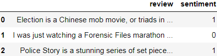

df.loc[0, 'review']

df.loc[0, 'review'][-50:]

     As you can see here, the text contains HTML markup as well as punctuation and other non-letter characters. While HTML markup does not contain many useful semantics, punctuation marks can represent useful, additional information in certain NLP contexts. However, for simplicity, we will now remove all punctuation marks except for emoticon characters, such as :), since those are certainly useful for sentiment analysis. To accomplish this task, we will use Python's regular expression (regex) library, re, as shown here:

Regular expressions

cp2 Advanced HTML Parsing( including Regexpression ) : cp2 Advanced HTML Parsing( including Regexpression )_Linli522362242的专栏-CSDN博客

03_Classification_02_confusion matrix _.reshape([-1])_score(average="macro")_interpolation.shift正则表达 : 03_Classification_2_regex_confusion matrix_.reshape([-1])_score(average=“macro“)_interpolation.shift_Linli522362242的专栏-CSDN博客

MySQL_max_min_count_like_distinct_(CHAR_LENGTH)_RIGHT(Name, 3) asc_UNION ALL_RLIKE_(regexp)_CaseWhen : MySQL_max_min_count_like_distinct_(CHAR_LENGTH)_RIGHT(Name, 3) asc_UNION ALL_RLIKE_(regexp)_CaseWhen_Linli522362242的专栏-CSDN博客

cp9_p172 2-grams OR N-grams From Sentences_re.sub: cp9_p172 2-grams OR N-grams From Sentences_re.sub_Linli522362242的专栏-CSDN博客

[^a-z]   负值字符范围。匹配任何不在指定范围内的任意字符。例如，“[^a-z]”可以匹配任何不在“a”到“z”范围内的任意字符。

re.sub('<[^>]*>', 
       '', 
       'is seven.<br >/><br />Title (Brazil): Not Available')

(?:pattern)   非获取匹配，匹配pattern但不获取匹配结果，不进行存储供以后使用。这在使用或字符“(|)”来组合一个模式的各个部分时很有用。例如“industr(?:y|ies)”就是一个比“industry|industries”更简略的表达式。 

re.findall( '(?::|;|=)', 'is seven.Title (Brazil): Not Available;=-')

re.findall( '(?::|;|=)(?:-)', 'is seven.Title (Brazil): Not Available;=-' )

 # Must meet 2 conditions at the same time： (?::|;|=) and (?:-)

re.findall( '(?::|;|=)(?:-)', 'is seven.Title (Brazil):- Not Available;=-' )

?   匹配前面的子表达式零次或一次。例如，“do(es)?”可以匹配“do”或“does”。?等价于{0,1}。

     当该字符紧跟在任何一个其他限制符（*,+,?，{n}，{n,}，{n,m}）后面时，匹配模式是非贪婪的。非贪婪模式尽可能少地匹配所搜索的字符串，而默认的贪婪模式则尽可能多地匹配所搜索的字符串。例如，对于字符串“oooo”，“o+”将尽可能多地匹配“o”，得到结果[“oooo”]，而“o+?”将尽可能少地匹配“o”，得到结果 ['o', 'o', 'o', 'o']

re.findall( '(?::|;|=)(?:-)?', 'is seven.Title (Brazil):- Not Available;=-' )

 #the conditions are met ：(?::|;|=) OR  (?::|;|=) and (?:-)

re.findall( '(?::|;|=)(?:-)?', 'is seven.Title (Brazil):- Not Available;=-;' )

re.findall( '(?::|;|=)(?:-)?', 'is seven.Title (Brazil):- Not Available;=--' )

re.findall( '(?::|;|=)(?:-)?(?:\)|\()', 'is seven.Title (Brazil):- Not Available;=-)' )

#the conditions are met ：   (?::|;|=) and (?:-) and (?:\)|\() 

                                                        OR  (?::|;|=)                and (?:\)|\()  

re.findall( '(?::|;|=)(?:-)?(?:\)|\()', 'is seven.Title (Brazil):- Not Available;=)' )

re.findall( '(?::|;|=)(?:-)?(?:\)|\(|D|P)', 'is seven.Title (Brazil):- Not Available;=)' )

#the conditions are met ：      (?::|;|=) and (?:-) and (?:\)|\(|D|P) 

                                                        OR  (?::|;|=)                and (?:\)|\(|D|P)  

' '.join( re.findall( '(?::|;|=)(?:-)?(?:\)|\(|D|P)', 'is seven.Title (Brazil):- Not Available;=)' )
        ).replace('-', '')

join :  convert a list to string with '  '  and '  ' as a kind of delimiter分隔符
then replace '-' with '' OR remove '-'

 

\W Capital W: 匹配任何非单词字符。等价于“[^A-Za-z0-9_]”。
\w 匹配包括下划线的任何单词字符。类似但不等价于“[A-Za-z0-9_]”，这里的"单词"字符使用Unicode字符集。
+   匹配前面的子表达式一次或多次(大于等于1次）。例如，“zo+”能匹配“zo”以及“zoo”，但不能匹配“z”。+等价于{1,}。

re.sub( '[\W]+', ' ', # [\W]+ : [^A-Za-z0-9_]+
                     'is seven.Title (Brazil):- Not Available;=)'.lower()
                   )

myTuple = ["John", "Peter", "Vicky"]

x = "#".join(myTuple)

print(x)

myTuple = []

x = "#".join(myTuple)

print(x)

# empty

myTuple = ['+']

x = "#".join(myTuple)

print(x)

myTuple = '+'

x = "#".join(myTuple)

print(x)

myTuple = '+'

x = "#".join(myTuple).replace('-', '')

print(x)

  

import re

def preprocessor(text):
    text = re.sub( '<[^>]*>', '', 
                   text) #remove html tag: <a>, <br />
    print(text)
    emoticons = re.findall( '(?::|;|=)(?:-)?(?:\)|\(|D|P)', 
                           text)
    print(emoticons)
    # ' '.join(emoticons) is not empty then .replace('-', '')
    print(' '.join(emoticons).replace('-', ''))
    text = ( re.sub( '[\W]+', ' ', # [\W]+ == [^A-Za-z0-9_]+ # [^A-Za-z0-9_] : '(' or ')' or ':'
                     text.lower() # replace any [^A-Za-z0-9_] with ' '
                   ) +
             ' '.join(emoticons).replace('-', '') # put the emoticons at the end
           )
    return text

preprocessor('is seven.<br /><br />Title (Brazil): Not Available')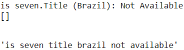

preprocessor( "</a>This :) is :( a test : -)!" )

1. remove html tag or markup: </a>
2. find all : #the conditions are met #      (?::|;|=) and (?:-) and (?:\)|\(|D|P)
                                                          OR  (?::|;|=)                and (?:\)|\(|D|P)  ==> ":)" and ":("
3. replace any [^A-Za-z0-9_] with ' ' OR remove any character in [A-Za-z0-9_] ==>  '   :)  ' and '  : -)!' and '  ' are removed

emoticons [iˈməutikɔnz] 情感符

df.loc[0, 'review'][-50:]

 

import re

def preprocessor(text):
    text = re.sub( '<[^>]*>', '', 
                   text) #remove html tag: <a>, <br />
    emoticons = re.findall( '(?::|;|=)(?:-)?(?:\)|\(|D|P)', 
                           text)
    text = ( re.sub( '[\W]+', ' ', # [\W]+ == [^A-Za-z0-9_]+ # [^A-Za-z0-9_] : '(' or ')' or ':'
                     text.lower() # replace any [^A-Za-z0-9_] with ' '
                   ) +
             ' '.join(emoticons).replace('-', '')# put the emoticons at the end
           )
    return text

preprocessor( df.loc[0, 'review'][-50:] )

     Via the first regex, <[^>]*>, in the preceding code section, we tried to remove all of the HTML markup from the movie reviews. Although many programmers generally
advise against the use of regex to parse HTML, this regex should be sufficient to clean this particular dataset. Since we are only interested in removing HTML markup and do not plan to use the HTML markup further, using regex to do the job should be acceptable. However, if you prefer using sophisticated tools for removing HTML markup from text, you can take a look at Python's HTML parser module, which is described at https://docs.python.org/3/library/html.parser.html. After we removed the HTML markup, we used a slightly more complex regex to find emoticons, which we temporarily stored as emoticons. Next, we removed all non-word characters from the text via the regex [\W]+ and converted the text into lowercase characters.

     Eventually, we added the temporarily stored emoticons to the end of the processed document string. Additionally, we removed the nose character (- in :-)) from the
emoticons for consistency.

##################################################

Dealing with word capitalization

     In the context of this analysis, we assume that the capitalization of a word—for example, whether it appears at the beginning of a sentence—does not contain semantically relevant information. However, note that there are exceptions; for instance, we remove the notation of proper names我们删除了专有名称的表示法. But again, in the context of this analysis, it is a simplifying assumption that the letter case does not contain information that is relevant for sentiment analysis.

Regular expressions

     Although regular expressions offer an efficient and convenient approach to searching for characters in a string, they also come with a steep learning curve. Unfortunately, an in-depth discussion of regular expressions is beyond the scope of this book. However, you can find a great tutorial on the Google Developers portal at https://developers.google.com/edu/python/regular-expressions or you can check out the official documentation of Python's re module at https://docs.python.org/3.7/library/re.html.

##################################################
     Although the addition of the emoticon characters to the end of the cleaned document strings may not look like the most elegant approach, we must note that the order of the words doesn't matter in our bag-of-words model if our vocabulary consists of only one-word tokens. But before we talk more about the splitting of documents into individual terms, words, or tokens, let's confirm that our preprocessor function works correctly:

preprocessor( "</a>This :) is :( a test : -)!" )

1. remove html tag or markup: </a>
2. find all : #the conditions are met #      (?::|;|=) and (?:-) and (?:\)|\(|D|P)
                                                          OR  (?::|;|=)                and (?:\)|\(|D|P)  ==> ":)" and ":("
3. replace any [^A-Za-z0-9_] with ' ' OR remove any character in [A-Za-z0-9_] ==>  '   :)  ' and '  : -)!' and '  ' are removed

     Lastly, since we will make use of the cleaned text data over and over again during the next sections, let's now apply our preprocessor function to all the movie reviews in our DataFrame:

df['review'] = df['review'].apply(preprocessor)

Processing documents into tokens

     After successfully preparing the movie review dataset, we now need to think about how to split the text corpora[ˈkɔrpərə]资料，文集，汇编（ corpus的名词复数 ） into individual elements. One way to tokenize标记化 documents is to split them into individual words by splitting the cleaned documents at their whitespace characters:

def tokenizer(text):
    return text.split()

tokenizer('runners like running and thus they run')

 

     In the context of tokenization, another useful technique is 词干提取word stemming['stemɪŋ]封堵; 遏止, which is the process of transforming a word into its root form. It allows us to map related words to the same stem. The original stemming algorithm was developed by Martin F. Porter in 1979 and is hence known as the Porter stemmer algorithm (An algorithm for suffix stripping, Martin F. Porter, Program: Electronic Library and Information Systems, 14(3): 130–137, 1980). The Natural Language Toolkit (NLTK, http://www.nltk.org) for Python implements the Porter stemming algorithm, which we will use in the following code section. In order to install the NLTK, you can simply execute conda install nltk or pip install nltk.

Installing NLTK(Natural Language Toolkit) : Installing NLTK — NLTK 3.6.2 documentation

Install_tensorflow_ notebook_ Spyder_tfgraphviz_pydot_Pandas_scikit-learn_ipython_pillow_NLTK : Instal_tf_notebook_Spyder_tfgraphviz_pydot_pd_scikit-learn_ipython_pillow_NLTK_flask_mlxtend_gym_mkl_Linli522362242的专栏-CSDN博客

NLTK online book
     Although the NLTK is not the focus of this chapter, I highly recommend that you visit the NLTK website as well as read the official NLTK book, which is freely available at
http://www.nltk.org/book/, if you are interested in more advanced applications in NLP.

def tokenizer(text):
    return text.split()

tokenizer('runners like running and thus they run')

 

The following code shows how to use the Porter stemming algorithm:

from nltk.stem.porter import PorterStemmer

porter = PorterStemmer()

def tokenizer_porter(text):
    return [porter.stem(word) for word in text.split()]

tokenizer_porter('runners like running and thus they run')

     Using the PorterStemmer from the nltk package, we modified our tokenizer function to reduce words to their root form, which was illustrated by the simple preceding example where the word 'running' was stemmed to its root form 'run'.

Stemming algorithms

     The Porter stemming algorithm is probably the oldest and simplest stemming algorithm. Other popular stemming algorithms include the newer Snowball stemmer (Porter2 or English stemmer) and the Lancaster stemmer (Paice/Huskstemmer). While both the Snowball and Lancaster stemmers are faster than the original Porter stemmer, the Lancaster stemmer is also notorious for being more aggressive than the Porter stemmer. These alternative stemming algorithms are also available through the NLTK package (http://www.nltk.org/api/nltk.stem.html).

     While stemming can create non-real words, such as 'thu' (from 'thus'), as shown in the previous example, a technique called lemmatization词形还原 aims to obtain the canonical (grammatically correct) forms of individual words—the socalled lemmas. However, lemmatization is computationally more difficult and expensive compared to stemming and, in practice, it has been observed that stemming and lemmatization have little impact on the performance of text classification (Influence of Word Normalization on Text Classification, Michal Toman, Roman Tesar, and Karel Jezek, Proceedings of InSciT, pages 354–358, 2006).

     Lemmatization词形还原 is another different process to reduce the dimensionality. In lemmatization process, it brings down the word to root word rather than just truncating the words. For example, bring ate to its root word as eat when we pass the ate word into lemmatizer with the POS tag as verb.

     Before we jump into the next section, where we will train a machine learning model using the bag-of-words model, let's briefly talk about another useful topic called stop-word removal停用词移除. Stop-words are simply those words that are extremely common in all sorts of texts and probably bear no (or only a little) useful information that can be used to distinguish between different classes of documents. Examples of stopwords are is, and, has, and so on. Removing stop-words can be useful if we are working with raw or normalized term frequencies rather than tf-idfs(可以用于减轻特征向量中这些频繁出现的单词的权重。), which are already downweighting frequently occurring words.
 For example: I, me, you, this, that, and so on, which needs to be removed before
further processing.

     In order to remove stop-words from the movie reviews, we will use the set of 127 English stop-words that is available from the NLTK library, which can be obtained
by calling the nltk.download function:

import nltk

nltk.download('stopwords')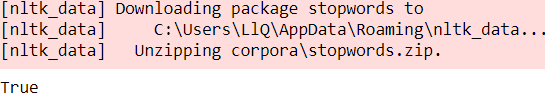

from nltk.corpus import stopwords

stop = stopwords.words('english')
[ w for w in tokenizer_porter('a runner likes running and runs a lot')
  if w not in stop]

Stop word removal<==Stemming of words<== original text('a runner likes running and runs a lot')

Training a logistic regression model for document classification

Obtaining the movie review dataset(Crawling, download, uncompression) ==>Preprocessing the movie dataset into a more convenient format(DataFrame)==>Cleaning text data(regex)

df.head()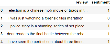

df.describe()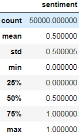

     In this section, we will train a logistic regression model to classify the movie reviews into positive and negative reviews based on the bag-of-words model. First, we will
divide the DataFrame of cleaned text documents into 25,000 documents for training and 25,000 documents for testing:

X_train = df.loc[:25000, 'review'].values
y_train = df.loc[:25000, 'sentiment'].values

X_test = df.loc[25000:, 'review'].values
y_test = df.loc[25000:, 'sentiment'].values

Next, we will use a GridSearchCV object to find the optimal set of parameters for our logistic regression model using 5-fold stratified cross-validation:

sklearn.feature_extraction.text.TfidfVectorizer sklearn.feature_extraction.text.TfidfVectorizer — scikit-learn 0.24.2 documentation
                      Convert a collection of raw documents to a matrix of TF-IDF features.
                      Equivalent to CountVectorizer followed by TfidfTransformer.

• strip_accents : {‘ascii’, ‘unicode’}, default=None
                            Remove accents重音 and perform other character normalization during the preprocessing step. ‘ascii’ is a fast method that only works on characters that have an direct ASCII mapping. ‘unicode’ is a slightly slower method that works on any characters. None (default) does nothing.
                            Both ‘ascii’ and ‘unicode’ use NFKD normalization from unicodedata.normalize.

• lowercase : bool, default=True
                       Convert all characters to lowercase before tokenizing( text.split() ).
• preprocessor : callable, default=None

                            Override the preprocessing (string transformation) stage while preserving the tokenizing and n-grams generation steps. Only applies if analyzer is notcallable.

• ngram_range : tuple (min_n, max_n), default=(1, 1)

                            The lower and upper boundary of the range of n-values for different n-grams to be extracted. All values of n such that min_n <= n <= max_n will be used. For example an ngram_range of (1, 1) means only unigrams单元组, (1, 2) means unigrams and bigrams二元组, and (2, 2) means only bigrams. Only applies if analyzer is not callable.

• stop_words : {‘english’}, list, default=None
                         If a string, it is passed to _check_stop_list and the appropriate stop list is returned. ‘english’ is currently the only supported string value. There are several known issues with ‘english’ and you should consider an alternative (see Using stop words, stop words : probably bear no (or only a little) useful information that can be used to distinguish between different classes of documents, Examples of stopwords are is, and, has, and like).

                         If a list, that list is assumed to contain stop words, all of which will be removed from the resulting tokens. Only applies if analyzer == 'word'.

                         If None, no stop words will be used. max_df can be set to a value in the range [0.7, 1.0) to automatically detect and filter stop words based on intra corpus document frequency of terms.

• tokenizer ： callable, default=None
                       Override the string tokenization step while preserving the preprocessing and n-grams generation steps. Only applies if analyzer == 'word'.

• analyzer ：{‘word’, ‘char’, ‘char_wb’} or callable, default=’word’

                     Whether the feature should be made of word or character n-grams. Option ‘char_wb’ creates character n-grams only from text inside word boundaries; n-grams at the edges of words are padded with space.

                    If a callable is passed it is used to extract the sequence of features out of the raw, unprocessed input.

• Using Google colab

!pip install -U -q PyDrive 
  
from pydrive.auth import GoogleAuth 
from pydrive.drive import GoogleDrive 
from google.colab import auth 
from oauth2client.client import GoogleCredentials 
  
  
# Authenticate and create the PyDrive client. 
auth.authenticate_user() 
gauth = GoogleAuth() 
gauth.credentials = GoogleCredentials.get_application_default() 
drive = GoogleDrive(gauth)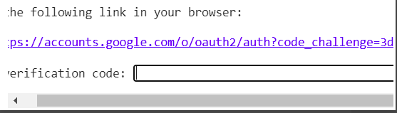

==>
  ==>
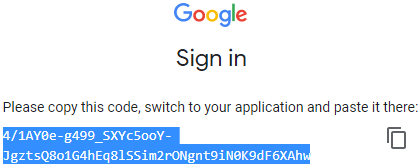
4/1AY0e-g499_SXYc5ooY-JgztsQ8o1G4hEq8lSSim2rONgnt9iN0K9dF6XAhw

Click on the link prompted to get the authentication to allow Google to access your Drive. You will see a screen with “Google Cloud SDK wants to access your Google Account” at the top. After you allow permission, copy the given verification code and paste it in the box in Colab. 

Now, go to the CSV file in your Drive and get the shareable link and store it in a string variable in Colab.

==>==>copy link

Now, to get this file in dataframe run the following code.

link = "https://drive.google.com/file/d/1ZvAU59qTx66mstqF5tpeKCEHj2MlqwxR/view?usp=sharing"

import pandas as pd 
  
# to get the id part of the file 
id = link.split("/")[-2] 
  
downloaded = drive.CreateFile({'id':id})  
downloaded.GetContentFile('movie_data.csv')   
  
df = pd.read_csv('movie_data.csv') 
print(df)

import re

def preprocessor(text):
    text = re.sub( '<[^>]*>', '', 
                   text) #remove html tag: <a>, <br />
    emoticons = re.findall( '(?::|;|=)(?:-)?(?:\)|\(|D|P)', 
                           text)
    text = ( re.sub( '[\W]+', ' ', # [\W]+ == [^A-Za-z0-9_]+ # [^A-Za-z0-9_] : '(' or ')' or ':'
                     text.lower() # replace any [^A-Za-z0-9_] with ' '
                   ) +
             ' '.join(emoticons).replace('-', '')# put the emoticons at the end
           )
    return text

    preprocessor( df.loc[0, 'review'][-50:] )

def tokenizer(text):
    return text.split()

from nltk.stem.porter import PorterStemmer

porter = PorterStemmer()

def tokenizer_porter(text):
    return [porter.stem(word) for word in text.split()]


import nltk

nltk.download('stopwords')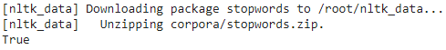

from nltk.corpus import stopwords

stop = stopwords.words('english')
[ w for w in tokenizer_porter('a runner likes running and runs a lot')
  if w not in stop]

X_train = df.loc[:25000, 'review'].values
y_train = df.loc[:25000, 'sentiment'].values

X_test = df.loc[25000:, 'review'].values
y_test = df.loc[25000:, 'sentiment'].values

Next, we will use a GridSearchCV object to find the optimal set of parameters for our logistic regression model using 5-fold stratified cross-validation:

sklearn.feature_extraction.text.TfidfVectorizer sklearn.feature_extraction.text.TfidfVectorizer — scikit-learn 0.24.2 documentation
                      Convert a collection of raw documents to a matrix of TF-IDF features.
                      Equivalent to CountVectorizer followed by TfidfTransformer.

• strip_accents : {‘ascii’, ‘unicode’}, default=None
                            Remove accents重音 and perform other character normalization during the preprocessing step. ‘ascii’ is a fast method that only works on characters that have an direct ASCII mapping. ‘unicode’ is a slightly slower method that works on any characters. None (default) does nothing.
                            Both ‘ascii’ and ‘unicode’ use NFKD normalization from unicodedata.normalize.

• lowercase : bool, default=True
                       Convert all characters to lowercase before tokenizing( text.split() ).
• preprocessor : callable, default=None

                            Override the preprocessing (string transformation) stage while preserving the tokenizing and n-grams generation steps. Only applies if analyzer is notcallable.

• ngram_range : tuple (min_n, max_n), default=(1, 1)

                            The lower and upper boundary of the range of n-values for different n-grams to be extracted. All values of n such that min_n <= n <= max_n will be used. For example an ngram_range of (1, 1) means only unigrams单元组, (1, 2) means unigrams and bigrams二元组, and (2, 2) means only bigrams. Only applies if analyzer is not callable.

• stop_words : {‘english’}, list, default=None
                         If a string, it is passed to _check_stop_list and the appropriate stop list is returned. ‘english’ is currently the only supported string value. There are several known issues with ‘english’ and you should consider an alternative (see Using stop words, stop words : probably bear no (or only a little) useful information that can be used to distinguish between different classes of documents, Examples of stopwords are is, and, has, and like).

                         If a list, that list is assumed to contain stop words, all of which will be removed from the resulting tokens. Only applies if analyzer == 'word'.

                         If None, no stop words will be used. max_df can be set to a value in the range [0.7, 1.0) to automatically detect and filter stop words based on intra corpus document frequency of terms.

• tokenizer ： callable, default=None
                       Override the string tokenization step while preserving the preprocessing and n-grams generation steps. Only applies if analyzer == 'word'.

• analyzer ：{‘word’, ‘char’, ‘char_wb’} or callable, default=’word’

                     Whether the feature should be made of word or character n-grams. Option ‘char_wb’ creates character n-grams only from text inside word boundaries; n-grams at the edges of words are padded with space.

                    If a callable is passed it is used to extract the sequence of features out of the raw, unprocessed input.

from sklearn.pipeline import Pipeline
from sklearn.linear_model import LogisticRegression
from sklearn.feature_extraction.text import TfidfVectorizer
from sklearn.model_selection import GridSearchCV

tfidf = TfidfVectorizer( strip_accents=None, 
                         lowercase=False, 
                         preprocessor=None 
                       ) # combines CountVectorizer with the TfidfTransformer
#create new dataset: each_column__each_feature ~~ each_row_tf_idf_value_for each document

param_grid = [{'vect__ngram_range':[(1,1)], # 1-gram # step4:CountVectorizer ==> TfidfTransformer
               'vect__stop_words': [stop, None],     # step3:remove stop-word
               'vect__tokenizer': [tokenizer,        # step1:text.split
                                  tokenizer_porter],# step2:reduce words to their root form
               'clf__penalty':['l1', 'l2'],
               'clf__C':[1.0, 10.0, 100.0]
              }, 
              {'vect__ngram_range':[(1,1)],
               'vect__stop_words': [stop, None],
               'vect__tokenizer': [tokenizer,
                                  tokenizer_porter],
               'vect__use_idf':[False],
               'vect__norm':[None],
               'clf__penalty':['l1', 'l2'],
               'clf__C': [1.0, 10.0, 100.0]
              },
             ]

lr_tfidf = Pipeline([ ('vect', tfidf), #vectorization
                      ('clf', LogisticRegression(random_state=0, solver='liblinear')),
                    ])
gs_lr_tfidf = GridSearchCV(lr_tfidf, param_grid,
                           scoring='accuracy',
                           cv=5,
                           verbose=2,
                           n_jobs=-1
                           )

gs_lr_tfidf.fit(X_train, y_train)

 Multiprocessing via the n_jobs parameter

     Please note that it is highly recommended to set n_jobs=-1 (instead of n_jobs=1) in the previous code example to utilize all available cores on your machine and speed up the grid search. However, some Windows users reported issues when running the previous code with the n_jobs=-1 setting related to pickling the tokenizer and tokenizer_porter functions for multiprocessing on Windows. Another workaround would be to replace those two functions, [tokenizer, tokenizer_porter], with [str.split]. However, note that replacement by the simple str.split would not support stemming.

     When we initialized the GridSearchCV object and its parameter grid using the preceding code, we restricted ourselves to a limited number of parameter combinations, since the number of feature vectors, as well as the large vocabulary, can make the grid search computationally quite expensive. Using a standard desktop computer, our grid search may take up to 40 minutes to complete(>=40 minutes).

     In the previous code example, we replaced CountVectorizer and TfidfTransformer from the previous subsection with TfidfVectorizer, which combines CountVectorizer with the TfidfTransformer. Our param_grid consisted of two parameter dictionaries. In the first dictionary, we used TfidfVectorizer with its default settings (use_idf=True, smooth_idf=True, and  norm='l2') to calculate the tf-idfs; in the second dictionary, we set those parameters to use_idf=False, smooth_idf=False, and norm=None in order to train a model based on raw term frequencies. Furthermore, for the logistic regression classifier itself, we trained models using L2 and L1 regularization via the penalty parameter and compared different regularization strengths by defining a range of values for the inverse-regularization parameter C.

     After the grid search has finished, we can print the best parameter set:

print('Best parameter set: %s ' % gs_lr_tfidf.best_params_)
print('CV Accuracy: %.3f' % gs_lr_tfidf.best_score_)

Best parameter set: {'clf__C': 100.0, 'clf__penalty': 'l2', 'vect__ngram_range': (1, 1), 'vect__stop_words': None, 'vect__tokenizer': <function tokenizer at 0x7f74e1dc7378>}

CV Accuracy: 0.888 

     As you can see in the preceding output, we obtained the best grid search results using the regular tokenizer without Porter stemming, no stop-word library, and
tf-idfs in combination with a logistic regression classifier that uses L2-regularization with the regularization strength C of 100.0. 

     Using the best model from this grid search, let's print the average 5-fold crossvalidation accuracy scores on the training dataset and the classification accuracy
on the test dataset

clf = gs_lr_tfidf.best_estimator_
print('Test Accuracy: %.3f' % clf.score(X_test, y_test))

 

The results reveal that our machine learning model can predict whether a movie review is positive or negative with 90 percent accuracy.

The naïve Bayes classifier

      A still very popular classifier for text classification is the naïve Bayes classifier, which gained popularity in applications of email spam filtering. Naïve Bayes classifiers are easy to implement, computationally efficient, and tend to perform particularly well on relatively small datasets compared to other algorithms. Although we don't discuss naïve Bayes classifiers in this book, the interested reader can find an article about naïve Bayes text classification that is freely available on arXiv (Naive Bayes and Text Classification I – Introduction and Theory, S. Raschka, Computing Research Repository (CoRR), abs/1410.5329, 2014, http://arxiv.org/pdf/1410.5329v3.pdf).

The following I just used first dict and run code injupyter notebook

from sklearn.pipeline import Pipeline
from sklearn.linear_model import LogisticRegression
from sklearn.feature_extraction.text import TfidfVectorizer
from sklearn.model_selection import GridSearchCV

tfidf = TfidfVectorizer( strip_accents=None, 
                         lowercase=False, 
                         preprocessor=None 
                       ) # combines CountVectorizer with the TfidfTransformer
#create new dataset: each_column__each_feature ~~ each_row_tf_idf_value_for each document

param_grid = [{'vect__ngram_range':[(1,1)], # 1-gram # step4:CountVectorizer ==> TfidfTransformer
               'vect__stop_words': [stop, None],     # step3:remove stop-word
               'vect__tokenizer': [tokenizer,        # step1:text.split
                                  tokenizer_porter],# step2:reduce words to their root form
               'clf__penalty':[ 'l1', 'l2'],
               'clf__C':[1.0, 10.0, 100.0]
              }, 
#               {'vect__ngram_range':[(1,1)],
#                'vect__stop_words': [stop, None],
#                'vect__tokenizer': [tokenizer,
#                                   tokenizer_porter],
#                'vect__use_idf':[False],
#                'vect__norm':[None],
#                'clf__penalty':['l2'],
#                'clf__C': [10.0]
#               },
             ]

lr_tfidf = Pipeline([ ('vect', tfidf), #vectorization
                      ('clf', LogisticRegression(random_state=0, solver='liblinear')),
                    ])
gs_lr_tfidf = GridSearchCV(lr_tfidf, param_grid,
                           scoring='accuracy',
                           cv=5,
                           verbose=2,
                           n_jobs=-1
                           )

gs_lr_tfidf.fit(X_train, y_train)

 

     Please note that gs_lr_tfidf.best_score_ is the average k-fold cross-validation score. I.e., if we have a GridSearchCV object with 5-fold cross-validation (like the one above), the best_score_ attribute returns the average score over the 5-folds of the best model.

print('Best parameter set: %s ' % gs_lr_tfidf.best_params_)
print('CV Accuracy: %.3f' % gs_lr_tfidf.best_score_)

     As you can see in the preceding output, we obtained the best grid search results using the regular tokenizer without Porter stemming, no stop-word library, and
tf-idfs in combination with a logistic regression classifier that uses L2-regularization with the regularization strength C of 10.0. 

Thus, I suggest when running the code(the grid search computationally quite expensive) in which will cost a lot time, you should figure out a solution to split your code(run your code piece by piece) or reduce your code running time

clf = gs_lr_tfidf.best_estimator_
print('Test Accuracy: %.3f' % clf.score(X_test, y_test))

The results reveal that our machine learning model can predict whether a movie review is positive or negative with 90 percent accuracy.

     Please note that gs_lr_tfidf.best_score_ is the average k-fold cross-validation score. I.e., if we have a GridSearchCV object with 5-fold cross-validation (like the one above), the best_score_ attribute returns the average score over the 5-folds of the best model. To illustrate this with an example:

from sklearn.linear_model import LogisticRegression
import numpy as np

from sklearn.model_selection import StratifiedKFold
from sklearn.model_selection import cross_val_score

np.random.seed(0)
np.set_printoptions(precision=6)
y = [np.random.randint(3) for i in range(25)]
# y ==> [0, 1, 0, 1, 1, 2, 0, 2, 0, 0, 0, 2, 1, 2, 2, 0, 1, 1, 1, 1, 0, 1, 0, 0, 1]
# np.array(y).shape ==>(25,) # 1D array with 25 columns
       # np.random.randn(25).reshape(-1,1).shape ==>(25, 1) # 2D array with 25 rows 1 column
X = (y + np.random.randn(25).reshape(-1,1))
# since len(y)==25, so call np.random.randn(25).reshape(-1,1) 25 times then each column+y_element
# (y+np.random.randn(25).reshape(-1,1)).shape ==> (25, 25)
cv5_idx = list( StratifiedKFold(n_splits=5, shuffle=False).split(X,y) )

lr = LogisticRegression(random_state=123, multi_class='ovr', solver='lbfgs')
cross_val_score(lr, X, y, cv=cv5_idx)

X[:3]

cv5_idx

     By executing the code above, we created a simple data set of random integers that shall represent our class labels. Next, we fed the indices of 5 cross-validation folds (cv5_idx) to the cross_val_score scorer, which returned 5 accuracy scores -- these are the 5 accuracy values for the 5 test folds.

cross_val_score(lr, X, y, cv=cv5_idx).mean()

 

Next, let us use the GridSearchCV object and feed it the same 5 cross-validation sets (via the pre-generated cv5_idx indices):

from sklearn.model_selection import GridSearchCV

lr = LogisticRegression( solver='lbfgs', multi_class='ovr', random_state=1 )
gs = GridSearchCV( lr, {}, cv=cv5_idx, verbose=5 ).fit(X,y)

 

As we can see, the scores for the 5 folds are exactly the same as the ones from cross_val_score earlier.

Now, the bestscore attribute of the GridSearchCV object, which becomes available after fitting, returns the average accuracy score of the best model

gs.best_score_

######################################################################################
verbose = 0 为不在标准输出流输出日志信息
verbose = 1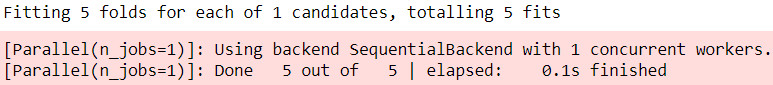 

verbose = 2 输出2行记录

verbose = 3 输出3行记录

######################################################################################

Working with bigger data – online algorithms and out-of-core learning

    If you executed the code examples in the previous section, you may have noticed that it could be computationally quite expensive to construct the feature vectors for the 50,000-movie review dataset during grid search. In many real-world applications, it is not uncommon to work with even larger datasets that can exceed our computer's memory. Since not everyone has access to supercomputer facilities, we will now apply a technique called out-of-core learning, which allows us to work with such large datasets by fitting the classifier incrementally on smaller batches of a dataset.

Text classification with recurrent neural networks

     In Chapter 16, Modeling Sequential Data Using Recurrent Neural Networks, we will revisit this dataset and train a deep learningbased classifier (a recurrent neural network) to classify the reviews in the IMDb movie review dataset. This neural networkbased classifier follows the same out-of-core principle using the stochastic gradient descent optimization algorithm but does not require the construction of a bag-of-words model.

     Back in Cp2, Training Simple Machine Learning Algorithms for Classification cp2_TrainingSimpleMachineLearningAlgorithmsForClassification_meshgrid_ravel_contourf_OvA_GradientDes_Linli522362242的专栏-CSDN博客, the concept of stochastic gradient descent随机梯度下降(also referred to as batch gradient descent) was introduced; it is an optimization algorithm that updates the model's weights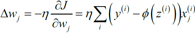 using one example at a time. In this section, we will make use of the partial_fit function of SGDClassifier in scikitlearn to stream the documents directly from our local drive and train a logistic regression model using small mini-batches of documents.

# This cell is not contained in the book but
# added for convenience so that the notebook
# can be executed starting here
import os
import gzip


if not os.path.isfile('movie_data.csv'):
    if not os.path.isfile('movie_data.csv.gz'):
        print('Please place a copy of the movie_data.csv.gz'
              'in this directory. You can obtain it by'
              'a) executing the code in the beginning of this'
              'notebook or b) by downloading it from GitHub:'
              'https://github.com/rasbt/python-machine-learning-'
              'book-2nd-edition/blob/master/code/ch08/movie_data.csv.gz')
    else:
        with gzip.open('movie_data.csv.gz', 'rb') as in_f, \
                open('movie_data.csv', 'wb') as out_f:
            out_f.write(in_f.read())

     First, we will define a tokenizer function that cleans the unprocessed text data from the movie_data.csv file that we constructed at the beginning of this chapter and separate it into word tokens while removing stop-words: 

import numpy as np
import re
from nltk.corpus import stopwords

import nltk

nltk.download('stopwords')

# stop-words probably bear no (or only a little) useful information that 
# can be used to distinguish between different classes of documents
stop = stopwords.words('english')

def tokenizer(text):
    text = re.sub('<[^>]*>', '', text) # remove html markup : <a>, <br />
    emoticons = re.findall( '(?::|;|=)(?:-)?(?:\)|\(|D|P)',
                           text.lower())
    text = re.sub( '[\W]+', ' ', # [\w]+ == [^A-Za-z0-9_]* : '(' or ')' 
                   text.lower() 
                 ) + ' '.join(emoticons).replace('-', '') # put the emoticons at the end
    return text

Next, we will define a generator function, stream_docs, that reads in and returns one document at a time:

def stream_docs(path):
    with open(path, 'r', encoding='utf-8') as csv:
        next(csv) #skip header
        for line in csv:
            text, label = line[:-3], int(line[-2]) # line[-1] : EOF
            yield text, label

     To verify that our stream_docs function works correctly, let's read in the first document from the movie_data.csv file, which should return a tuple consisting of the review text as well as the corresponding class label: 

next(stream_docs(path='movie_data.csv'))

     We will now define a function, get_minibatch, that will take a document stream from the stream_docs function and return a particular number of documents specified by the size parameter:

def get_minibatch(doc_stream, size):
    docs, y= [], []
    try:
        for _ in range(size):
            text, label = next(doc_stream)
            docs.append(text)
            y.append(label)
    except StopIteration:
        return None, None
    return docs, y

     Unfortunately, we can't use CountVectorizer for out-of-core learning since it requires holding the complete vocabulary in memory. Also, TfidfVectorizer needs to keep all the feature vectors of the training dataset in memory to calculate the inverse document frequencies. However, another useful vectorizer for text processing implemented in scikit-learn is HashingVectorizer. HashingVectorizer is data-independent and makes use of the hashing trick via the 32-bit MurmurHash3 function by Austin Appleby (https://sites.google.com/site/murmurhash/):

sklearn.feature_extraction.text.HashingVectorizer

sklearn.feature_extraction.text.HashingVectorizer — scikit-learn 0.24.2 documentation

Convert a collection of text documents to a matrix of token occurrences

It turns a collection of text documents into a scipy.sparse matrix holding token occurrence counts (or binary occurrence information), possibly normalized as token frequencies if norm=’l1’ or projected on the euclidean unit sphere if norm=’l2’.

This text vectorizer implementation uses the hashing trick to find the token string name to feature integer index mapping.

This strategy has several advantages:

• it is very low memory scalable to large datasets as there is no need to store a vocabulary dictionary in memory

• it is fast to pickle and un-pickle as it holds no state besides the constructor parameters

• it can be used in a streaming (partial fit) or parallel pipeline as there is no state computed during fit.

There are also a couple of cons (vs using a CountVectorizer with an in-memory vocabulary):

• there is no way to compute the inverse transform (from feature indices to string feature names) which can be a problem when trying to introspect which features are most important to a model.

• there can be collisions: distinct tokens can be mapped to the same feature index. However in practice this is rarely an issue if n_features is large enough (e.g. 2 ** 18 for text classification problems).

• no IDF weighting as this would render the transformer stateful.

The hash function employed is the signed 32-bit version of Murmurhash3.

Using the preceding code, we initialized HashingVectorizer with our tokenizer function and set the number of features to 2**21.

from sklearn.feature_extraction.text import HashingVectorizer
from sklearn.linear_model import SGDClassifier

vect = HashingVectorizer( decode_error='ignore', 
                         n_features=2**21, 
                         preprocessor=None, 
                         tokenizer=tokenizer)

     Furthermore, we reinitialized a logistic regression classifier by setting the loss parameter of SGDClassifier to 'log'. Note that by choosing a large number of features in HashingVectorizer, we reduce the chance of causing hash collisions, but we also increase the number of coefficients in our logistic regression model.

clf = SGDClassifier( loss='log', random_state=1 )
doc_stream = stream_docs( path='movie_data.csv' )

loss :  str, default=’hinge’  05_Support Vector Machines_hinge_support vectors_decision function_Lagrange multiplier拉格朗日乘数_C~slack_Linli522362242的专栏-CSDN博客

         The loss function to be used. Defaults to ‘hinge’, which gives a linear SVM. The possible options are ‘hinge’, ‘log’, ‘modified_huber’, ‘squared_hinge’, ‘perceptron’, or a regression loss: ‘squared_loss’, ‘huber’, ‘epsilon_insensitive’, or ‘squared_epsilon_insensitive’.

        The ‘log’ loss gives logistic regression, a probabilistic classifier. ‘modified_huber’ is another smooth loss that brings tolerance to outliers as well as probability estimates. ‘squared_hinge’ is like hinge but is quadratically penalized. ‘perceptron’ is the linear loss used by the perceptron algorithm. The other losses are designed for regression but can be useful in classification as well; see SGDRegressor for a description.

Now comes the really interesting part – having set up all the complementary functions, we can start the out-of-core learning using the following code:

partial_fit(X, y, classes=None, sample_weight=None) : Perform one epoch of stochastic gradient descent on given samples.

                                                                                             Internally, this method uses max_iter = 1. Therefore, it is not guaranteed that a minimum of the cost function is reached after calling it once. Matters such as objective convergence and early stopping should be handled by the user.

import pyprind
pbar = pyprind.ProgBar(45)

classes = np.array([0,1])
for _ in range(45):
    X_train, y_train = get_minibatch( doc_stream, size=1000 )
    if not X_train:
        break
    X_train = vect.transform(X_train)
    clf.partial_fit(X_train, y_train, classes=classes)
    pbar.update()

     Again, we made use of the PyPrind package in order to estimate the progress of our learning algorithm. We initialized the progress bar object with 45 iterations and, in the following for loop, we iterated over 45 mini-batches of documents where each mini-batch consists of 1,000 documents.

Having completed the incremental learning process, we will use the last 5,000 documents to evaluate the performance of our model:

X_test, y_test = get_minibatch( doc_stream, size=5000)
X_test = vect.transform(X_test)
print( 'Accuracy: %.3f' % clf.score(X_test, y_test))

TypeError: 'NoneType' object is not iterable

Solution: Please run your code from where you defined HashingVectorizer ( decode_error='ignore',  n_features=2**21,  preprocessor=None, tokenizer=tokenizer)

     As you can see, the accuracy of the model is 61 percent, slightly below the accuracy that we achieved in the previous section using the grid search for hyperparameter tuning. However, out-of-core learning is very memory efficient and it took less than a minute to complete. Finally, we can use the last 5,000 documents to update our model:

The word2vec model

     A more modern alternative to the bag-of-words model is word2vec, an algorithm that Google released in 2013 (Efficient Estimation of Word Representations in Vector Space, T. Mikolov, K. Chen, G. Corrado, and J. Dean, arXiv preprint arXiv:1301.3781, 2013). 

     The word2vec algorithm is an unsupervised learning algorithm based on neural networks that attempts to automatically learn the relationship between words. The idea behind word2vec is to put words that have similar meanings into similar clusters, and via clever vector-spacing, the model can reproduce certain
words using simple vector math, for example, king – man +woman = queen.

     The original C-implementation with useful links to the relevant papers and alternative implementations can be found at https://code.google.com/p/word2vec/.

Topic modeling with Latent Dirichlet Allocation

     Topic modeling describes the broad task of assigning topics to unlabeled text documents. For example, a typical application would be the categorization of documents in a large text corpus of newspaper articles. In applications of topic modeling, we then aim to assign category labels to those articles, for example, sports, finance, world news, politics, local news, and so forth. Thus, in the context of the broad categories of machine learning that we discussed in Chapter 1, Giving Computers the Ability to Learn from Data #1_from Statistics to ML_agent_policy_explanatory_predictor_response_numeric_mode_Hypothesis_Chi-squ_Linli522362242的专栏-CSDN博客, we can consider topic modeling as a clustering task, a subcategory of unsupervised learning.

     In this section, we will discuss a popular technique for topic modeling called Latent Dirichlet狄利克雷的 Allocation (LDA). However, note that while Latent Dirichlet Allocation is often abbreviated as LDA, it is not to be confused with linear discriminant判别式 analysis cp5_Compressing Data via Dimensionality Reduction_feature extraction_PCA_LDA_convergence_kernel PCA_Linli522362242的专栏-CSDN博客, a supervised dimensionality reduction technique that was introduced in Chapter 5, Compressing Data via Dimensionality Reduction.

     Embedding the movie review classifier into a web application LDA is different from the supervised learning approach that we took in this chapter to classify movie reviews as positive and negative. Thus, if you are interested in embedding scikit-learn models into a web application via the Flask framework using the movie reviewer as an example, please feel free to jump to the next chapter and revisit this standalone section on topic modeling later on.

Decomposing text documents with LDA

     Since the mathematics behind LDA is quite involved and requires knowledge about Bayesian inference, we will approach this topic from a practitioner's perspective and interpret LDA using layman's terms. However, the interested reader can read more about LDA in the following research paper: Latent Dirichlet Allocation, David M. Blei, Andrew Y. Ng, and Michael I. Jordan, Journal of Machine Learning Research 3, pages: 993-1022, Jan 2003.

     LDA is a generative probabilistic model that tries to find groups of words that appear frequently together across different documents. These frequently appearing
words represent our topics, assuming that each document is a mixture of different words. The input to an LDA is the bag-of-words model that we discussed earlier in this chapter. Given a bag-of-words matrix as input, LDA decomposes it into two new matrices:

• • A document-to-topic matrix
• • A word-to-topic matrix

     LDA decomposes the bag-of-words matrix in such a way that if we multiply those two matrices together, we will be able to reproduce the input, the bag-of-words matrix, with the lowest possible error. In practice, we are interested in those topics that LDA found in the bag-of-words matrix. The only downside may be that we must define the number of topics beforehand—the number of topics is a hyperparameter of LDA that has to be specified manually.

LDA with scikit-learn

     In this subsection, we will use the LatentDirichletAllocation class implemented in scikit-learn to decompose the movie review dataset and categorize it into different
topics. In the following example, we will restrict the analysis to 10 different topics, but readers are encouraged to experiment with the hyperparameters of the algorithm to further explore the topics that can be found in this dataset.

     First, we are going to load the dataset into a pandas DataFrame using the local movie_data.csv file of the movie reviews that we created at the beginning of this chapter:

import pandas as pd

df =  pd.read_csv('movie_data.csv', encoding='utf-8')
df.head(3)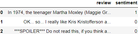

Next, we are going to use the already familiar CountVectorizer to create the bag-ofwords matrix as input to the LDA.

For convenience, we will use scikit-learn's built-in English stop-word library via stop_words='english':

from sklearn.feature_extraction.text import CountVectorizer

count = CountVectorizer( stop_words='english',
                         max_df=.1,
                         max_features=5000 )
X = count.fit_transform(df['review'].values)
X.shape

     Notice that we set the maximum document frequency of words to be considered to 10 percent (max_df=.1) to exclude words that occur too frequently across documents. The rationale behind the removal of frequently occurring words is that these might be common words appearing across all documents that are, therefore, less likely to be associated with a specific topic category of a given document. Also, we limited the number of words to be considered to the most frequently occurring 5,000 words (max_features=5000), to limit the dimensionality of this dataset to improve the inference performed by LDA. However, both max_df=.1 and max_features=5000 are hyperparameter values chosen arbitrarily, and readers are encouraged to tune them while comparing the results.

     The following code example demonstrates how to fit a LatentDirichletAllocation estimator to the bag-of-words matrix and infer the 10 different topics from the
documents (note that the model fitting can take up to 5 minutes or more on a laptop or standard desktop computer):

from sklearn.decomposition import LatentDirichletAllocation
lda = LatentDirichletAllocation( n_components=10, 
                                 random_state=123, 
                                 learning_method='batch' 
                               )
X_topics = lda.fit_transform(X) # get topics for some given samples:
X_topics.shape

 

X_topics[:3]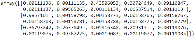

 

     By setting learning_method='batch', we let the lda estimator do its estimation based on all available training data (the bag-of-words matrix) in one iteration, which is slower than the alternative 'online' learning method but can lead to more accurate results (setting learning_method='online' is analogous to online or minibatch
learning, which we discussed in Chapter 2, Training Simple Machine Learning Algorithms for Classification, and in this chapter).

Expectation-Maximization

     The scikit-learn library's implementation of LDA (Latent Dirichlet狄利克雷的 Allocation) uses the expectation-maximization (EM) 08_09_3_Dimensionality Reduction_Mixture Models and EM_K-means_Image segmentation_compression_Linli522362242的专栏-CSDN博客 algorithm to update its parameter estimates iteratively. We haven't discussed the EM algorithm in this chapter, but if you are curious to learn more, please see the excellent overview on Wikipedia (https://en.wikipedia.org/wiki/Expectation-maximization_algorithm) and the detailed tutorial on how it is used in LDA in Colorado Reed's tutorial, Latent Dirichlet Allocation: Towards a Deeper Understanding, which is freely available at http://obphio.us/pdfs/lda_tutorial.pdf.

     After fitting the LDA, we now have access to the components_ attribute of the lda instance, which stores a matrix containing the word importance (here, 5000) for each of the 10 topics in increasing order:  #A word-to-topic matrixA word-to-topic matrix

lda.components_.shape

 10 topics ~ 5000 same words or same features

     To analyze the results, let's print the five most important words for each of the 10 topics. Note that the word importance values are ranked in increasing order.
Thus, to print the top five words, we need to sort the topic array in reverse order:

n_top_words = 10
feature_names = count.get_feature_names()

for topic_idx, topic in enumerate(lda.components_):
    print( "Topic %d:" % (topic_idx+1) )
    print( " ".join([feature_names[i]
                     for i in topic.argsort()[:-n_top_words-1:-1]
                    ]) # argsort() : Returns the indices that would sort an array.
         )

Based on reading the 5 most important words for each topic, we may guess that the LDA identified the following topics:

1. Comedies
2. Generally bad movies (not really a topic category)
3. Movies somehow related to TV shows
4. Movies about families
5. War movies
6. Action movies
7. Movies based on books
8. Art movies
9. Horror movies恐怖电影
10. Animation

     To confirm that the categories make sense based on the reviews, let's plot three movies from the animation category (animation belong to category 10 at
index position 9):

# X_topics.shape : (50000 instances, 10 topics)
# the animation movie category (category 10 at index position 9)
animation = X_topics[:,9].argsort()[::-1]

for iter_idx, movie_idx in enumerate(animation[:3]): #first 3 movies
    print( "\nAnimation movie #%d:" % (iter_idx+1) )
    print( df['review'][movie_idx][:500], '...') #get first 500 words from reviews

     Using the preceding code example, we printed the first 500 characters from the top three Animation movies. The reviews—even though we don't know which exact movie they belong to—sound like reviews of Animation movies .

Summary

     In this chapter, you learned how to use machine learning algorithms to classify text documents based on their polarity, which is a basic task in sentiment analysis
in the field of NLP. Not only did you learn how to encode a document as a feature vector using the bag-of-words model, but you also learned how to weight the term frequency by relevance using tf-idf.

     Working with text data can be computationally quite expensive due to the large feature vectors that are created during this process; in the last section, we covered
how to utilize out-of-core or incremental learning to train a machine learning algorithm without loading the whole dataset into a computer's memory.

     Lastly, you were introduced to the concept of topic modeling using LDA to categorize the movie reviews into different categories in an unsupervised fashion.

     In the next chapter, we will use our document classifier and learn how to embed it into a web application.