机器学习-决策树算法

turbosqi

已于 2022-11-24 20:52:44 修改

阅读量1.6k

点赞数 2

分类专栏：机器学习文章标签：决策树算法

于 2022-11-24 20:20:37 首次发布

本文链接：https://blog.csdn.net/Lshuangye/article/details/128025005

版权

机器学习专栏收录该内容

8 篇文章 12 订阅

订阅专栏

机器学习-基础知识
机器学习-线性回归
机器学习-逻辑回归
机器学习-聚类算法
机器学习-决策树算法
机器学习-集成算法
机器学习-SVM算法

1. 决策树算法

1.1. 什么是决策树/判定树

决策树是一个类似于流程图的树结构，其中，每个内部结点表示在一个属性上的测试，每个分支代表一个属性输出，而每个树叶结点代表类或类的分布，树的顶层是根结点。决策树是一种有监督学习的一种算法，是机器学习中分类方法中的一个重要分支。

1.2. 决策树归纳算法

在这里插入图片描述

策略：
1. 自根至叶的递归过程，在每个中间结点寻找一个"划分"属性；
2. 开始构建根结点，所有训练数据都放在根结点，选择一个最优特征，按照这一特征将训练集分割成子集，进入子结点；
3. 所有子集按内部结点的属性递归的进行分割；
4. 如果这些子集已经能够被基本正确分类，那么构建叶结点，并将这些子集分到所对应的叶结点上去；
5. 每个子集都被分到叶结点上，即都有了明确的类，这就生成了一颗决策树。
三种停止条件：
1. 当前结点包含的样本全属于同一个类别，无需划分；
2. 当前属性集为空，或者所有样本在所有属性上取值相同，无法划分；
3. 当前结点包含的样本集合为空，不能划分。

1.3. 熵概念

用比特(bit)来衡量信息的多少

熵：
$\sum_{x}{P(x)log_2[P(x)]}\quad\quad\quad\quad\quad\quad\quad\quad\quad\quad\quad\quad\quad\quad\quad\quad\quad\quad\quad$
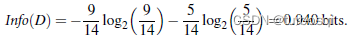
变量的不确定性越大，熵就越大。

信息的获取量：

$Infor_A(D)\quad\quad\quad\quad\quad\quad\quad\quad\quad\quad\quad\quad\quad\quad\quad\quad\quad$

1.4. 具体算法

ID3算法

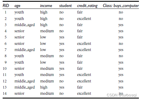
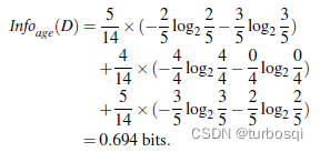
对于以上的四个属性中，最大的信息熵为age，所以选择age作为第一个分支，建立决策树
在这里插入图片描述

具体的实现过程：
在这里插入图片描述

CART算法

反映了从D中随机抽取两个样例，其类别标记不一致的概率

Gini(D)越小，数据集D的纯度越高
$Gini(D)=\sum_{k=1}^{|y|}\sum_{k^{'}\neq k}{p_kp_k{'}}=1-\sum_{k=1}^{|y|}{p_k^2} \quad\quad\quad\quad\quad\quad\quad\quad\quad\quad\quad\quad\quad$
属性a的基尼指数：
$Gini\_index(D,a)=\sum_{v=1}^{V}\frac{|D^v|}{|D|} Gini(D^v)\quad\quad\quad\quad\quad\quad\quad\quad\quad\quad\quad\quad\quad$
在候选属性集合中，选取那个使划分后基尼系数最小的属性
具体计算过程：
增益率-C4.5算法

信息增益：对可取值数目较多的属性有所偏好(缺点)
$Gini\_ratio(D,a)=\frac{Gain(D,a)}{IV(a)} \quad\quad\quad\quad\quad\quad\quad\quad\quad\quad\quad\quad\quad$
增益率：
$IV(a)=-\sum_{v=1}^{V}\frac{|D^v|}{|D|}log_2\frac{|D^v|}{|D|} \quad\quad\quad\quad\quad\quad\quad\quad\quad\quad\quad\quad\quad\quad\quad$
- 属性a的可能取值数目越大(即V越大)，则IV(a)的值通常就越大
- 启发式：先从候选划分属性中找出信息增益高于平均水平的，再从中选取增益率最高的

1.5. 决策树剪枝

剪枝：防止决策树过拟合
基本策略：
- 预剪枝：提前终止某些分支的生长
  
  限制深度，叶子结点个数，叶子结点的样本数，信息增益等
- 后剪枝：生成一棵完全树，再回头剪枝
  
  通过一定的衡量标准： $C_ \alpha (T)=C(T)+ \alpha \cdot |T_{leaf}|$
优缺点：
- 时间开销：
  - 预剪枝：训练时间开销降低，测试时间开销降低
  - 后剪枝：训练时间开销增加，测试时间开销降低
- 过/欠拟合风险：
  - 预剪枝：过拟合风险降低，欠拟合风险增加
  - 后剪枝：过拟合风险降低，欠拟合风险不变
- 泛化性能：
  
  后剪枝通常由于预剪枝

1.6. 连续值与缺失值处理

1.6.1. 连续值处理

连续值处理：由于连续属性的可取值数目不再有限，因此不能直接根据连续属性的可取值来对结点进行划分。
基本思路：连续属性离散化
常见做法：二分法

1.6.2. 缺失值处理

基本思路: 样本赋权，权重划分

1.7. 决策树算法的优缺点

优点：
1. 速度快：计算量相对较少，且容易转化为分类规则。只要沿着树根向下一直走到叶，沿途的分裂条件就能唯一确定一条分类的谓词。
2. 准确性高：挖掘出来的分类规则准确性高，便于理解，决策树可以清晰的看到哪些字段比较重要
3. 非参数学习，不需要设置参数
缺点：
1. 缺乏伸缩性：由于进行深度优先搜索，所以算法受内存大小限制，难于处理大训练集。
2. 为了处理大数据集或连续值的种种改进算法(离散化、取样)不仅增加了分类算法的额外开销，而且降低了分类的准确性,对连续性的字段比较难预测，当类别太多时，错误可能就会增加的比较快，对有时间顺序的数据，需要很多预处理的工作。

1.8. 决策树算法的具体实现

1.8.1. 使用sklearn工具包实现

from sklearn.feature_extraction import DictVectorizer
# 读取和写入csv文件时用到
import csv
# 导入决策树模块
from sklearn import tree
# 导入数据预处理模块
from sklearn import preprocessing


# 读取csv文件，并将特征放入dict列表和类标签列表中
allElectronicsData = open("注意：文件路径",'rt')
reader = csv.reader(allElectronicsData)
headers = next(reader)
print(headers)

# 保存前面的属性组
featureList = []
# 保存后面的标签分类
labelList = []

for row in reader:
    labelList.append(row[len(row)-1])
    rowDict = {}
    for i in range(1,len(row)-1):
        rowDict[headers[i]] = row[i]
    featureList.append(rowDict)
print(featureList)

# 数据预处理,把分类数据二值化
vec = DictVectorizer()
dummyx = vec.fit_transform(featureList).toarray()
print("dummyX:" + str(dummyx))
print(vec.get_feature_names_out())

print("labelList:" + str(labelList))
lb = preprocessing.LabelBinarizer()
dummyY = lb.fit_transform(labelList)
print("dummyY:" + str(dummyY))

# 创建决策树分类的对象
clf = tree.DecisionTreeClassifier(criterion='entropy')
clf = clf.fit(dummyx,dummyY)

# 可视化模型
with open("注意：文件路径", 'w') as f:
    f = tree.export_graphviz(clf, feature_names=vec.get_feature_names_out(), out_file=f)

# 测试集进行验证
oneRowW = dummyx[0,:]
print("oneRowX:" + str(oneRowW))

# 把数据集中的年龄改为中年
newRowX = oneRowW
newRowX[0] = 1
newRowX[2] = 0
print("newRowX:" + str(newRowX))

newRowX = [newRowX]
predictedY = clf.predict(newRowX)
print("predictedY:" + str(predictedY))

结果展示：
在这里插入图片描述

1.8.2. 模拟实现

导包操作

import matplotlib.pyplot as plt
from math import log
import operator

算法模拟核心

def createDataSet():
	dataSet = [[0, 0, 0, 0, 'no'],
			   [0, 0, 0, 1, 'no'],
			   [0, 1, 0, 1, 'yes'],
			   [0, 1, 1, 0, 'yes'],
			   [0, 0, 0, 0, 'no'],
			   [1, 0, 0, 0, 'no'],
			   [1, 0, 0, 1, 'no'],
			   [1, 1, 1, 1, 'yes'],
			   [1, 0, 1, 2, 'yes'],
			   [1, 0, 1, 2, 'yes'],
			   [2, 0, 1, 2, 'yes'],
			   [2, 0, 1, 1, 'yes'],
			   [2, 1, 0, 1, 'yes'],
			   [2, 1, 0, 2, 'yes'],
			   [2, 0, 0, 0, 'no']]
	labels = ['F1-AGE','F2-WORK','F3-HOME','F4-LOAN']
	return dataSet,labels

def createTree(dataset,labels,featLabels):
	"""
	dataset:数据集
	labels:最终的标签的分类
	featLabels: 标签的顺序
	"""
	# 把数据集最后一列的值存入classList
	classList = [example[-1] for example in dataset]

	# 当样本的标签全部一样时，就会相等
	if classList.count(classList[0]) == len(classList):
		return classList[0]
	# 当前数据集中只剩下一类标签，此时已经遍历完了所有的数据集
	if len(dataset[0]) == 1:
		return majorityCnt(classList)

	# 选择最优的特征,对应索引值
	bestFeat = chooseBestFeatureToSplit(dataset)
	# 找到实际的名字
	bestFeatLabel = labels[bestFeat]
	featLabels.append(bestFeatLabel)

	myTree = {bestFeatLabel:{}}
	del labels[bestFeat]


	featValue = [example[bestFeat] for example in dataset]
	# 得到不同的分支
	uniqueVals = set(featValue)
	for value in uniqueVals:
		# 递归运行过程中,标签值的更替
		sublabels = labels[:]
		myTree[bestFeatLabel][value] = createTree(splitDataSet(dataset,bestFeat,value),sublabels,featLabels)
	return myTree

def majorityCnt(classList):
	"""计算哪一个类最多的"""
	classCount = {}
	for vote in classList:
	   if vote not in classCount.keys():classCount[vote] = 0
	   classCount[vote] += 1
	# 排序后的结果
	sortedclassCount = sorted(classCount.items(),key=operator.itemgetter(1),reverse=True)
	return sortedclassCount[0][0]

def chooseBestFeatureToSplit(dataset):
	numFeatures = len(dataset[0]) - 1
	baseEntropy = calcShannonEnt(dataset)
	# 最好的信息增益
	bestInfoGain = 0
	# 最好的特征
	bestFeature = -1
	for i in range(numFeatures):
		featList = [example[i] for example in dataset]
		uniqueVals = set(featList)
		newEntropy = 0
		for val in uniqueVals:
			subDataSet = splitDataSet(dataset,i,val)
			prob = len(subDataSet)/float(len(dataset))
			newEntropy += prob * calcShannonEnt(subDataSet)
		infoGain = baseEntropy - newEntropy
		if infoGain > bestInfoGain:
			bestInfoGain = infoGain
			bestFeature = i
	return bestFeature


def splitDataSet(dataset,axis,val):
	retDataSet = []
	for featVec in dataset:
		if featVec[axis] == val:
			reducedFeatVec = featVec[:axis]
			reducedFeatVec.extend(featVec[axis+1:])
			retDataSet.append(reducedFeatVec)
	return retDataSet

def calcShannonEnt(dataset):
	"""最开始时候的熵值"""
	numexamples = len(dataset)
	labelCounts = {}
	# 先进行统计
	for featVec in dataset:
		currentlabel = featVec[-1]
		if currentlabel not in labelCounts.keys():
			labelCounts[currentlabel] = 0
		labelCounts[currentlabel] += 1

	shannonEnt = 0
	for key in labelCounts:
		prop = float(labelCounts[key])/numexamples
		shannonEnt -= prop*log(prop,2)
	return shannonEnt

画图操作

def getNumLeafs(myTree):
	numLeafs = 0
	firstStr = next(iter(myTree))
	secondDict = myTree[firstStr]
	for key in secondDict.keys():
		if type(secondDict[key]).__name__=='dict':
			numLeafs += getNumLeafs(secondDict[key])
		else:   numLeafs +=1
	return numLeafs


def getTreeDepth(myTree):
	maxDepth = 0
	firstStr = next(iter(myTree))
	secondDict = myTree[firstStr]
	for key in secondDict.keys():
		if type(secondDict[key]).__name__=='dict':
			thisDepth = 1 + getTreeDepth(secondDict[key])
		else:   thisDepth = 1
		if thisDepth > maxDepth: maxDepth = thisDepth
	return maxDepth

def plotNode(nodeTxt, centerPt, parentPt, nodeType):
	arrow_args = dict(arrowstyle="<-")
	#font = FontProperties(fname=r"c:\windows\fonts\simsunb.ttf", size=14)
	createPlot.ax1.annotate(nodeTxt, xy=parentPt,  xycoords='axes fraction',
		xytext=centerPt, textcoords='axes fraction',
		va="center", ha="center", bbox=nodeType, arrowprops=arrow_args)#, FontProperties=font


def plotMidText(cntrPt, parentPt, txtString):
	xMid = (parentPt[0]-cntrPt[0])/2.0 + cntrPt[0]
	yMid = (parentPt[1]-cntrPt[1])/2.0 + cntrPt[1]
	createPlot.ax1.text(xMid, yMid, txtString, va="center", ha="center", rotation=30)


def plotTree(myTree, parentPt, nodeTxt):
	decisionNode = dict(boxstyle="sawtooth", fc="0.8")
	leafNode = dict(boxstyle="round4", fc="0.8")
	numLeafs = getNumLeafs(myTree)
	depth = getTreeDepth(myTree)
	firstStr = next(iter(myTree))
	cntrPt = (plotTree.xOff + (1.0 + float(numLeafs))/2.0/plotTree.totalW, plotTree.yOff)
	plotMidText(cntrPt, parentPt, nodeTxt)
	plotNode(firstStr, cntrPt, parentPt, decisionNode)
	secondDict = myTree[firstStr]
	plotTree.yOff = plotTree.yOff - 1.0/plotTree.totalD
	for key in secondDict.keys():
		if type(secondDict[key]).__name__=='dict':
			plotTree(secondDict[key],cntrPt,str(key))
		else:
			plotTree.xOff = plotTree.xOff + 1.0/plotTree.totalW
			plotNode(secondDict[key], (plotTree.xOff, plotTree.yOff), cntrPt, leafNode)
			plotMidText((plotTree.xOff, plotTree.yOff), cntrPt, str(key))
	plotTree.yOff = plotTree.yOff + 1.0/plotTree.totalD


def createPlot(inTree):
	fig = plt.figure(1, facecolor='white')	
  #清空fig
	fig.clf()																				
	axprops = dict(xticks=[], yticks=[])
  #去掉x、y轴
	createPlot.ax1 = plt.subplot(111, frameon=False, **axprops)   
  #获取决策树叶结点数目
	plotTree.totalW = float(getNumLeafs(inTree))
  #获取决策树层数
	plotTree.totalD = float(getTreeDepth(inTree))			
  #x偏移
	plotTree.xOff = -0.5/plotTree.totalW; plotTree.yOff = 1.0		
  #绘制决策树
	plotTree(inTree, (0.5,1.0), '')															
	plt.show()

具体实现

if __name__ == '__main__':
	# 获取数据
	dataset,labels = createDataSet()
	featLabels = []
	mytree = createTree(dataset, labels, featLabels)
	createPlot(mytree)

结果展示

2. 决策树算法实践

2.1. 决策树实现步骤

导包操作

import numpy as np
import os
%matplotlib inline
import matplotlib
import matplotlib.pyplot as plt
plt.rcParams['axes.labelsize'] = 14
plt.rcParams['xtick.labelsize'] = 12
plt.rcParams['ytick.labelsize'] = 12
import warnings
warnings.filterwarnings('ignore')

加载数据集

导入燕尾花的数据集和决策树模型，并且加载数据集进行训练

from sklearn.datasets import load_iris
from sklearn.tree import DecisionTreeClassifier

iris = load_iris()
X = iris.data[:,2:]
y = iris.target

tree_clf = DecisionTreeClassifier(max_depth=2)
tree_clf.fit(X,y)

导出决策树模型

# 以DOT格式导出决策树
from sklearn.tree import export_graphviz

export_graphviz(
    tree_clf,
    out_file="iris_tree.dot",
    feature_names=iris.feature_names[2:],
    class_names=iris.target_names,
    rounded=True,
    filled=True
)

使用graphviz包中的dot命令行工具将此**.dot**文件转换为各种格式，如PDF或PNG QMDownload\ChromeDownload\iris tree.dot -o E:\QMDownload\ChromeDownload\iris_tree.png

决策树：dot -Tpdf iris.dot(源文件) -o output.pdf(目标文件)
加载树模型到Jupyter

# 把图片加载到jupyter
from IPython.display import Image
Image(filename='E:\QMDownload\ChromeDownload\iris_tree.png',width = 350,height = 350)

效果展示

2.2. 绘制决策边界

绘制图形

from matplotlib.colors import ListedColormap


def plot_decision_boundary(clf, X, y, axes=[0, 7.5, 0, 3], iris=True, legend=False, plot_training=True):
    x1s = np.linspace(axes[0], axes[1], 100)
    x2s = np.linspace(axes[2], axes[3], 100)
    x1, x2 = np.meshgrid(x1s, x2s)
    X_new = np.c_[x1.ravel(), x2.ravel()]
    y_pred = clf.predict(X_new).reshape(x1.shape)
    custom_cmap = ListedColormap(['#fafab0','#9898ff','#a0faa0'])
    plt.contourf(x1, x2, y_pred, alpha=0.3, cmap=custom_cmap)
    if not iris:
        custom_cmap2 = ListedColormap(['#7d7d58','#4c4c7f','#507d50'])
        plt.contour(x1, x2, y_pred, cmap=custom_cmap2, alpha=0.8)
    if plot_training:
        plt.plot(X[:, 0][y==0], X[:, 1][y==0], "yo", label="Iris-Setosa")
        plt.plot(X[:, 0][y==1], X[:, 1][y==1], "bs", label="Iris-Versicolor")
        plt.plot(X[:, 0][y==2], X[:, 1][y==2], "g^", label="Iris-Virginica")
        plt.axis(axes)
    if iris:
        plt.xlabel("Petal length", fontsize=14)
        plt.ylabel("Petal width", fontsize=14)
    else:
        plt.xlabel(r"$x_1$", fontsize=18)
        plt.ylabel(r"$x_2$", fontsize=18, rotation=0)
    if legend:
        plt.legend(loc="lower right", fontsize=14)

        
plt.figure(figsize=(8, 4))
plot_decision_boundary(tree_clf, X, y)
plt.plot([2.45, 2.45], [0, 3], "k-", linewidth=2)
plt.plot([2.45, 7.5], [1.75, 1.75], "k--", linewidth=2)
plt.plot([4.95, 4.95], [0, 1.75], "k:", linewidth=2)
plt.plot([4.85, 4.85], [1.75, 3], "k:", linewidth=2)
plt.text(1.40, 1.0, "Depth=0", fontsize=15)
plt.text(3.2, 1.80, "Depth=1", fontsize=13)
plt.text(4.05, 0.5, "(Depth=2)", fontsize=11)
plt.title('Decision Tree decision boundaries')

plt.show()

效果展示

从此图中能够看出，当Depth=0时，分的横轴Petal length，以2.45为标准，当Petal length<2.45时，class=setosa，大于的时候是另外两类；然后以纵轴Petal width划分，当Petal width<1.75时，class=versicolor，大于1.75时是class=virginica

2.3. 概率估计

估计类概率
输入数据为：花瓣长5厘米，宽1.5厘米的花。相应的叶节点是深度为2的左节点，因此决策树应输出以下概率：

Iris-Setosa 为 0％（0/54）
Iris-Versicolor 为 90.7％（49/54）
Iris-Virginica 为 9.3％（5/54）

# 预测概率值
tree_clf.predict_proba([[5,1.5]])
## 结果：array([[0. , 0.90740741, 0.09259259]])

# 直接预测结果
tree_clf.predict([[5,1.5]])
## 结果：array([1])

2.4. 决策树中的正则化

通过DecisionTreeClassifier类的一些参数来设置，防止出现决策树过拟合的现象，下面列出五种常用的参数以及代表的含义

min_samples_split ：节点在分割之前必须具有的最小样本数
min_samples_leaf ：叶子节点必须具有的最小样本数
max_leaf_nodes ：叶子节点的最大数量
max_features ：在每个节点处评估用于拆分的最大特征数
max_depth ：树最大的深度

五种参数的具体实现

# 测试案例
from sklearn.datasets import make_moons
X,y = make_moons(n_samples = 100,noise = 0.25,random_state = 53)
tree_clf1 = DecisionTreeClassifier(random_state=42)
tree_clf2 = DecisionTreeClassifier(min_samples_split=20,random_state=42)
tree_clf3 = DecisionTreeClassifier(min_samples_leaf=4,random_state=42)
tree_clf4 = DecisionTreeClassifier(max_leaf_nodes=20,random_state=42)
tree_clf5 = DecisionTreeClassifier(max_features=2,random_state=42)
tree_clf6 = DecisionTreeClassifier(max_depth=5,random_state=42)
tree_clf1.fit(X,y)
tree_clf2.fit(X,y)
tree_clf3.fit(X,y)
tree_clf4.fit(X,y)
tree_clf5.fit(X,y)
tree_clf6.fit(X,y)

plt.figure(figsize=(18,11))
plt.subplot(231)
plot_decision_boundary(tree_clf1,X,y,axes=[-1.5,2.5,-1,1.5],iris = False)
plt.title('Origin image')

plt.subplot(232)
plot_decision_boundary(tree_clf2,X,y,axes=[-1.5,2.5,-1,1.5],iris = False)
plt.title('min_samples_split=20')

plt.subplot(233)
plot_decision_boundary(tree_clf3,X,y,axes=[-1.5,2.5,-1,1.5],iris = False)
plt.title('min_samples_leaf=4')

plt.subplot(234)
plot_decision_boundary(tree_clf4,X,y,axes=[-1.5,2.5,-1,1.5],iris = False)
plt.title('max_leaf_nodes=20')

plt.subplot(235)
plot_decision_boundary(tree_clf5,X,y,axes=[-1.5,2.5,-1,1.5],iris = False)
plt.title('max_features=2')

plt.subplot(236)
plot_decision_boundary(tree_clf6,X,y,axes=[-1.5,2.5,-1,1.5],iris = False)
plt.title('max_depth=5')

效果展示

从图像上看，当min_samples_split=20和min_samples_leaf=4的时候效果较好，其他都出现过拟合的现象，在测试集上的表现相对较差。

2.5. 决策树对数据敏感

代码实例

np.random.seed(6)
Xs = np.random.rand(100, 2) - 0.5
ys = (Xs[:, 0] > 0).astype(np.float32) * 2

angle = np.pi / 4
rotation_matrix = np.array([[np.cos(angle), -np.sin(angle)], [np.sin(angle), np.cos(angle)]])
Xsr = Xs.dot(rotation_matrix)

tree_clf_s = DecisionTreeClassifier(random_state=42)
tree_clf_s.fit(Xs, ys)
tree_clf_sr = DecisionTreeClassifier(random_state=42)
tree_clf_sr.fit(Xsr, ys)

plt.figure(figsize=(11, 4))
plt.subplot(121)
plot_decision_boundary(tree_clf_s, Xs, ys, axes=[-0.7, 0.7, -0.7, 0.7], iris=False)
plt.title('Sensitivity to training set rotation')

plt.subplot(122)
plot_decision_boundary(tree_clf_sr, Xsr, ys, axes=[-0.7, 0.7, -0.7, 0.7], iris=False)
plt.title('Sensitivity to training set rotation')

plt.show()

效果展示

左图是原始图像以及分类的结果；右图为左图向右旋转90度后的结果，可以看出，决策树并不是简单的画一条斜线，而是出现连续的线段。

2.6. 回归任务

2.6.1. 回归任务

模拟数据集

np.random.seed(42)
m=200
X=np.random.rand(m,1)
y = 4*(X-0.5)**2
y = y + np.random.randn(m,1)/10

进行训练

from sklearn.tree import DecisionTreeRegressor

tree_reg = DecisionTreeRegressor(max_depth=2)
tree_reg.fit(X,y)

导出决策树模型

export_graphviz(
        tree_reg,
        out_file=("regression_tree.dot"),
        feature_names=["x1"],
        rounded=True,
        filled=True
    )

加载树模型到Jupyter

# 把图片加载到jupyter
from IPython.display import Image
Image(filename='E:/QMDownload/ChromeDownload/regression_tree.png',width = 450,height = 600)

结果展示

2.6.2. 树的深度影响

from sklearn.tree import DecisionTreeRegressor

# 对比树的最大深度
tree_reg1 = DecisionTreeRegressor(random_state=42, max_depth=2)
tree_reg2 = DecisionTreeRegressor(random_state=42, max_depth=3)
tree_reg1.fit(X, y)
tree_reg2.fit(X, y)

def plot_regression_predictions(tree_reg, X, y, axes=[0, 1, -0.2, 1], ylabel="$y$"):
    x1 = np.linspace(axes[0], axes[1], 500).reshape(-1, 1)
    y_pred = tree_reg.predict(x1)
    plt.axis(axes)
    plt.xlabel("$x_1$", fontsize=18)
    if ylabel:
        plt.ylabel(ylabel, fontsize=18, rotation=0)
    plt.plot(X, y, "b.")
    plt.plot(x1, y_pred, "r.-", linewidth=2, label=r"$\hat{y}$")

plt.figure(figsize=(11, 4))
plt.subplot(121)
plot_regression_predictions(tree_reg1, X, y)
for split, style in ((0.1973, "k-"), (0.0917, "k--"), (0.7718, "k--")):
    plt.plot([split, split], [-0.2, 1], style, linewidth=2)
plt.text(0.21, 0.65, "Depth=0", fontsize=15)
plt.text(0.01, 0.2, "Depth=1", fontsize=13)
plt.text(0.65, 0.8, "Depth=1", fontsize=13)
plt.legend(loc="upper center", fontsize=18)
plt.title("max_depth=2", fontsize=14)

plt.subplot(122)
plot_regression_predictions(tree_reg2, X, y, ylabel=None)
for split, style in ((0.1973, "k-"), (0.0917, "k--"), (0.7718, "k--")):
    plt.plot([split, split], [-0.2, 1], style, linewidth=2)
for split in (0.0458, 0.1298, 0.2873, 0.9040):
    plt.plot([split, split], [-0.2, 1], "k:", linewidth=1)
plt.text(0.3, 0.5, "Depth=2", fontsize=13)
plt.title("max_depth=3", fontsize=14)

plt.show()

效果展示：

树的深度为3的时候，在0.0到0.2之间出现过拟合现象
在这里插入图片描述

2.6.3. 树的最小叶子结点个数影响

tree_reg1 = DecisionTreeRegressor(random_state=42)
tree_reg2 = DecisionTreeRegressor(random_state=42, min_samples_leaf=10)
tree_reg1.fit(X, y)
tree_reg2.fit(X, y)

x1 = np.linspace(0, 1, 500).reshape(-1, 1)
y_pred1 = tree_reg1.predict(x1)
y_pred2 = tree_reg2.predict(x1)

plt.figure(figsize=(11, 4))

plt.subplot(121)
plt.plot(X, y, "b.")
plt.plot(x1, y_pred1, "r.-", linewidth=2, label=r"$\hat{y}$")
plt.axis([0, 1, -0.2, 1.1])
plt.xlabel("$x_1$", fontsize=18)
plt.ylabel("$y$", fontsize=18, rotation=0)
plt.legend(loc="upper center", fontsize=18)
plt.title("No restrictions", fontsize=14)

plt.subplot(122)
plt.plot(X, y, "b.")
plt.plot(x1, y_pred2, "r.-", linewidth=2, label=r"$\hat{y}$")
plt.axis([0, 1, -0.2, 1.1])
plt.xlabel("$x_1$", fontsize=18)
plt.title("min_samples_leaf={}".format(tree_reg2.min_samples_leaf), fontsize=14)

plt.show()