


仅用Python实现一个两层的全连接网络
我认为此任务的难点在于反向传播那块的代码,以前对反向传播认识比较浅显,亲手推算后,才真正理解了反向传播,我已把反向传播这块做了补充,详情见
http://blog.csdn.net/margretwg/article/details/64920405(softmax梯度推导)
http://blog.csdn.net/margretwg/article/details/66974869(反向传播)
【2层神经网络类】
import numpy as np
import matplotlib.pyplot as plt


class TwoLayerNet(object):
  """
  A two-layer fully-connected neural network. The net has an input dimension of
  N, a hidden layer dimension of H, and performs classification over C classes.
  We train the network with a softmax loss function and L2 regularization on the
  weight matrices. The network uses a ReLU nonlinearity after the first fully
  connected layer.

  In other words, the network has the following architecture:

  input - fully connected layer - ReLU - fully connected layer - softmax

  The outputs of the second fully-connected layer are the scores for each class.
  """

  def __init__(self, input_size, hidden_size, output_size, std=1e-4):
    """
    Initialize the model. Weights are initialized to small random values and
    biases are initialized to zero. Weights and biases are stored in the
    variable self.params, which is a dictionary with the following keys:

    W1: First layer weights; has shape (D, H)
    b1: First layer biases; has shape (H,)
    W2: Second layer weights; has shape (H, C)
    b2: Second layer biases; has shape (C,)

    Inputs:
    - input_size: The dimension D of the input data.
    - hidden_size: The number of neurons H in the hidden layer.
    - output_size: The number of classes C.
    """
    self.params = {}
    self.params['W1'] = std * np.random.randn(input_size, hidden_size)
    self.params['b1'] = np.zeros(hidden_size)
    self.params['W2'] = std * np.random.randn(hidden_size, output_size)
    self.params['b2'] = np.zeros(output_size)

  def loss(self, X, y=None, reg=0.0):
    """
    Compute the loss and gradients for a two layer fully connected neural
    network.

    Inputs:
    - X: Input data of shape (N, D). Each X[i] is a training sample.
    - y: Vector of training labels. y[i] is the label for X[i], and each y[i] is
      an integer in the range 0 <= y[i] < C. This parameter is optional; if it
      is not passed then we only return scores, and if it is passed then we
      instead return the loss and gradients.
    - reg: Regularization strength.

    Returns:
    If y is None, return a matrix scores of shape (N, C) where scores[i, c] is
    the score for class c on input X[i].

    If y is not None, instead return a tuple of:
    - loss: Loss (data loss and regularization loss) for this batch of training
      samples.
    - grads: Dictionary mapping parameter names to gradients of those parameters
      with respect to the loss function; has the same keys as self.params.
    """
    # Unpack variables from the params dictionary
    W1, b1 = self.params['W1'], self.params['b1']
    W2, b2 = self.params['W2'], self.params['b2']
    N, D = X.shape

    # Compute the forward pass
    scores = None
    loss=0.0
    #############################################################################
    # TODO: Perform the forward pass, computing the class scores for the input. #
    # Store the result in the scores variable, which should be an array of      #
    # shape (N, C).                                                             #
    #############################################################################
    fc1=np.dot(X,W1)+b1 #N by H
    fc1_act=np.maximum(0,fc1)#relu
    fc2=np.dot(fc1_act,W2)+b2 #N by C
    scores=fc2

    #############################################################################
    #                              END OF YOUR CODE                             #
    #############################################################################
    # If the targets are not given then jump out, we're done
    if y is None:
      return scores

    # Compute the loss
    loss = None
    #############################################################################
    # TODO: Finish the forward pass, and compute the loss. This should include  #
    # both the data loss and L2 regularization for W1 and W2. Store the result  #
    # in the variable loss, which should be a scalar. Use the Softmax           #
    # classifier loss. So that your results match ours, multiply the            #
    # regularization loss by 0.5                                                #
    #############################################################################
    f_max = np.reshape(np.max(scores, axis=1), (N, 1))  # 找到每一行的最大值,然后reshape 之后减去
    # 这样可以防止后面的操作会出现数值上的一些偏差
    # regularization
    scores -= f_max #N BY C
    p = np.exp(scores) / np.sum(np.exp(scores), axis=1, keepdims=True)  # N by C #这里要注意,除的是每个样本的和,不能全求和
    # 求交叉熵!!
    y_true = np.zeros_like(p)
    y_true[np.arange(fc2.shape[0]), y] = 1.0  # 生成hot-vector
    loss = np.sum(-np.log(p[np.arange(N), y])) / N + 0.5 * reg * np.sum(W2*W2)+0.5 * reg * np.sum(W1*W1)
    #############################################################################
    #                              END OF YOUR CODE                             #
    #############################################################################
    # Backward pass: compute gradients
    grads = {}
    #############################################################################
    # TODO: Compute the backward pass, computing the derivatives of the weights #
    # and biases. Store the results in the grads dictionary. For example,       #
    # grads['W1'] should store the gradient on W1, and be a matrix of same size #
    #############################################################################
    #反向传播
    #先算scores的梯度
    dscores=p
    dscores[np.arange(N),y]-=1# 损失函数对fc2(xW+b),fc2的导数
    dscores/=N #N by C

    #Backprop into W2 and b2
    dW2=np.dot(fc1_act.T,dscores) #H by C
    db2=np.sum(dscores,axis=0,keepdims=True)# (1,C)

    #Backprop into hidden layer
    drelu=np.dot(dscores,W2.T)  #(N,H)
    dfc1=drelu
    dfc1[fc1<0]=0 #(N,H)
    #Backprop into W1 and b1
    db1=np.sum(dfc1,axis=0,keepdims=True) #(1,H)
    dW1=np.dot(X.T,dfc1) #(D,H)

    #Add regularization gradient contribution
    dW2+=reg*W2
    dW1+=reg*W1
    grads['W1']=dW1
    grads['W2']=dW2
    grads['b1']=db1
    grads['b2']=db2
    #############################################################################
    #                              END OF YOUR CODE                             #
    #############################################################################

    return loss, grads

  def train(self, X, y, X_val, y_val,
            learning_rate=1e-3, learning_rate_decay=0.95,
            reg=1e-5,mu=0.9,num_epochs=30, num_iters=100,
            batch_size=200, verbose=False):
    """
    Train this neural network using stochastic gradient descent.

    Inputs:
    - X: A numpy array of shape (N, D) giving training data.
    - y: A numpy array f shape (N,) giving training labels; y[i] = c means that
      X[i] has label c, where 0 <= c < C.
    - X_val: A numpy array of shape (N_val, D) giving validation data.
    - y_val: A numpy array of shape (N_val,) giving validation labels.
    - learning_rate: Scalar giving learning rate for optimization.
    - learning_rate_decay: Scalar giving factor used to decay the learning rate
      after each epoch.
    - reg: Scalar giving regularization strength.
    - num_iters: Number of steps to take when optimizing.
    - batch_size: Number of training examples to use per step.
    - verbose: boolean; if true print progress during optimization.
    """
    num_train = X.shape[0]
    iterations_per_epoch = int(max(num_train / batch_size, 1))

    # Use SGD to optimize the parameters in self.model
    loss_history = []
    train_acc_history = []
    val_acc_history = []

    for it in range(1,num_epochs*iterations_per_epoch+1):
      X_batch = None
      y_batch = None

      #########################################################################
      # TODO: Create a random minibatch of training data and labels, storing  #
      # them in X_batch and y_batch respectively.                             #
      #########################################################################
      choice=np.random.choice(num_train,batch_size,replace=True)
      #Sampling with relacement is faster than sampling without replacement
      #有重复比没重复更快
      X_batch=X[choice]
      y_batch=y[choice]

      #########################################################################
      #                             END OF YOUR CODE                          #
      #########################################################################

      # Compute loss and gradients using the current minibatch
      loss, grads = self.loss(X_batch, y=y_batch, reg=reg)# 得到的grad是个dict类型
      loss_history.append(loss)
      v_W2,v_b2,v_W1,v_b1=0.0,0.0,0.0,0.0


      #########################################################################
      # TODO: Use the gradients in the grads dictionary to update the         #
      # parameters of the network (stored in the dictionary self.params)      #
      # using stochastic gradient descent. You'll need to use the gradients   #
      # stored in the grads dictionary defined above.                         #
      ########################################################################
      #SGD
      '''for each_param in self.params:
        self.params[each_param] += -learning_rate*grads[each_param]'''

      #update with momentum
      v_W2=mu*v_W2-learning_rate*grads['W2']
      self.params['W2']+=v_W2
      v_W1 = mu * v_W1 - learning_rate * grads['W1']
      self.params['W1']+=v_W1
      v_b1 = mu * v_b1 - learning_rate * grads['b1']
      self.params['b1']+=np.squeeze(v_b1)
      v_b2 = mu * v_b2 - learning_rate * grads['b2']
      self.params['b2'] +=np.squeeze(v_b2)

      #########################################################################
      #                             END OF YOUR CODE                          #
      #########################################################################

      '''if verbose and it % 100 == 0:
        print ('iteration %d / %d: loss %f' % (it, num_iters, loss))'''

      # Every epoch, check train and val accuracy and decay learning rate.
      if it % iterations_per_epoch == 0:
        # Check accuracy
        epoch=it/iterations_per_epoch
        train_acc = (self.predict(X_batch) == y_batch).mean()
        val_acc = (self.predict(X_val) == y_val).mean()
        train_acc_history.append(train_acc)
        val_acc_history.append(val_acc)
        print('epoch %d/%d :loss %f, train_acc:%f, val_acc:%f'
              %(epoch,num_epochs,loss,train_acc,val_acc))

        # Decay learning rate
        learning_rate *= learning_rate_decay

    return {
      'loss_history': loss_history,
      'train_acc_history': train_acc_history,
      'val_acc_history': val_acc_history,
    }

  def predict(self, X):
    """
    Use the trained weights of this two-layer network to predict labels for
    data points. For each data point we predict scores for each of the C
    classes, and assign each data point to the class with the highest score.

    Inputs:
    - X: A numpy array of shape (N, D) giving N D-dimensional data points to
      classify.

    Returns:
    - y_pred: A numpy array of shape (N,) giving predicted labels for each of
      the elements of X. For all i, y_pred[i] = c means that X[i] is predicted
      to have class c, where 0 <= c < C.
    """
    y_pred = None

    ###########################################################################
    # TODO: Implement this function; it should be VERY simple!                #
    ###########################################################################
    score=self.loss(X)
    y_pred=np.argmax(score,axis=1)
    ###########################################################################
    #                              END OF YOUR CODE                           #
    ###########################################################################

    return y_pred
一、创建一个小网络用于检查
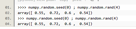
【补1】np.random.seed(0)
相当于设定一个随机的状态,当这个状态再次被调用时,随机数是一样的
#创建一个小网络来用作检查
#Note that we set the random seed for repeatable experiments

input_size=4
hidden_size=10
num_classes=3
num_inputs=5

def init_toy_model():
    np.random.seed(0)
    return TwoLayerNet(input_size,hidden_size,num_classesstd=1e-1)
def init_toy_data():
    np.random.seed(1)
    X=10*np.random.randn(num_inputs,input_size)#随机生成一个5*4的矩阵
    y=np.array([0,1,2,2,1])
    return X,y
net=init_toy_model()
X,y=init_toy_data()
前 向 传 播
scores=net.loss(X)#输入参数中没有y,则得到的是每个样本对应每个类别的分数
print('Your scores:')
print (scores)
print("correct scores:")
correct_scores=np.array([
  [-0.81233741, -1.27654624, -0.70335995],
  [-0.17129677, -1.18803311, -0.47310444],
  [-0.51590475, -1.01354314, -0.8504215 ],
  [-0.15419291, -0.48629638, -0.52901952],
  [-0.00618733, -0.12435261, -0.15226949]])
print (correct_scores)
print('Different between your scores and correct scores:')
print(np.sum(np.abs(scores-correct_scores)))

#算loss
loss,grad=net.loss(X,y,reg=0.1)
correct_loss=1.30378789133

print('Difference between your loss and correct loss:')
print(np.sum(np.abs(loss-correct_loss)))
梯 度 检 查
from cs231n.gradient_check import eval_numerical_gradient
for param_name in grad:
    f=lambda W: net.loss(X,y,reg=0.1)[0]
    param_grad_num=eval_numerical_gradient(f,net.params[param_name],verbose=False)
    print('%s max relative error: %e'%(param_name,rel_error(param_grad_num,grad[param_name])))
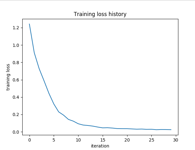
训练(向量法更新参数)
net=init_toy_model()
stats=net.train(X,y,X,y,learning_rate=1e-1,reg=1e-5,num_iters=100,verbose=False)#返回的是个dict

print('Final training loss:',stats['loss_history'][-1])
#plot the loss history
plt.plot(stats['loss_history'])
plt.xlabel('iteration')
plt.ylabel('training loss')
plt.title('Training loss history')
plt.show()
该模块输出结果为:
Your scores:
[[-0.81233741 -1.27654624 -0.70335995]
 [-0.17129677 -1.18803311 -0.47310444]
 [-0.51590475 -1.01354314 -0.8504215 ]
 [-0.15419291 -0.48629638 -0.52901952]
 [-0.00618733 -0.12435261 -0.15226949]]
correct scores:
[[-0.81233741 -1.27654624 -0.70335995]
 [-0.17129677 -1.18803311 -0.47310444]
 [-0.51590475 -1.01354314 -0.8504215 ]
 [-0.15419291 -0.48629638 -0.52901952]
 [-0.00618733 -0.12435261 -0.15226949]]
Different between your scores and correct scores:
3.68027204961e-08
Difference between your loss and correct loss:
1.79856129989e-13
b2 max relative error: 3.865091e-11
W2 max relative error: 3.440708e-09
b1 max relative error: 1.555470e-09
W1 max relative error: 3.561318e-09
epoch 1/30 :loss 1.241994, train_acc:0.660000, val_acc:0.600000
epoch 2/30 :loss 0.911191, train_acc:1.000000, val_acc:1.000000
epoch 3/30 :loss 0.727970, train_acc:1.000000, val_acc:1.000000
epoch 4/30 :loss 0.587932, train_acc:1.000000, val_acc:1.000000
epoch 5/30 :loss 0.443400, train_acc:1.000000, val_acc:1.000000
epoch 6/30 :loss 0.321233, train_acc:1.000000, val_acc:1.000000
epoch 7/30 :loss 0.229577, train_acc:1.000000, val_acc:1.000000
epoch 8/30 :loss 0.191958, train_acc:1.000000, val_acc:1.000000
epoch 9/30 :loss 0.142653, train_acc:1.000000, val_acc:1.000000
epoch 10/30 :loss 0.122731, train_acc:1.000000, val_acc:1.000000
epoch 11/30 :loss 0.092965, train_acc:1.000000, val_acc:1.000000
epoch 12/30 :loss 0.077945, train_acc:1.000000, val_acc:1.000000
epoch 13/30 :loss 0.072626, train_acc:1.000000, val_acc:1.000000
epoch 14/30 :loss 0.065361, train_acc:1.000000, val_acc:1.000000
epoch 15/30 :loss 0.054620, train_acc:1.000000, val_acc:1.000000
epoch 16/30 :loss 0.045523, train_acc:1.000000, val_acc:1.000000
epoch 17/30 :loss 0.047018, train_acc:1.000000, val_acc:1.000000
epoch 18/30 :loss 0.042983, train_acc:1.000000, val_acc:1.000000
epoch 19/30 :loss 0.037004, train_acc:1.000000, val_acc:1.000000
epoch 20/30 :loss 0.036127, train_acc:1.000000, val_acc:1.000000
epoch 21/30 :loss 0.036055, train_acc:1.000000, val_acc:1.000000
epoch 22/30 :loss 0.032943, train_acc:1.000000, val_acc:1.000000
epoch 23/30 :loss 0.030061, train_acc:1.000000, val_acc:1.000000
epoch 24/30 :loss 0.031595, train_acc:1.000000, val_acc:1.000000
epoch 25/30 :loss 0.028289, train_acc:1.000000, val_acc:1.000000
epoch 26/30 :loss 0.029215, train_acc:1.000000, val_acc:1.000000
epoch 27/30 :loss 0.024275, train_acc:1.000000, val_acc:1.000000
epoch 28/30 :loss 0.026362, train_acc:1.000000, val_acc:1.000000
epoch 29/30 :loss 0.025849, train_acc:1.000000, val_acc:1.000000
epoch 30/30 :loss 0.024548, train_acc:1.000000, val_acc:1.000000
Final training loss: 0.0245481639812
二、正式训练
1.读入数据
from cs231n.data_utils import load_CIFAR10
def get_CIFAR10_data(num_training=9000,num_validation=1000,num_test=1000):
    cifar10_dir='cs231n//datasets'
    X_train,y_train,X_test,y_test=load_CIFAR10(cifar10_dir)

    #subsample
    mask = range(num_training, num_training + num_validation)
    X_val = X_train[mask]
    y_val = y_train[mask]
    mask = range(num_training)
    X_train = X_train[mask]
    y_train = y_train[mask]
    mask = range(num_test)
    X_test = X_test[mask]
    y_test = y_test[mask]

    # Normalize the data: subtract the mean image
    mean_image = np.mean(X_train, axis=0)
    X_train -= mean_image
    X_val -= mean_image
    X_test -= mean_image

    # Reshape data to rows
    X_train = X_train.reshape(num_training, -1)
    X_val = X_val.reshape(num_validation, -1)
    X_test = X_test.reshape(num_test, -1)

    return X_train, y_train, X_val, y_val, X_test, y_test

# Invoke the above function to get our data.
X_train, y_train, X_val, y_val, X_test, y_test = get_CIFAR10_data()
print ('Train data shape: ', X_train.shape)
print ('Train labels shape: ', y_train.shape)
print ('Validation data shape: ', X_val.shape)
print ('Validation labels shape: ', y_val.shape)
print ('Test data shape: ', X_test.shape)
print ('Test labels shape: ', y_test.shape)
2.训练网络
input_size=32*32*3
hidden_size=50
num_classes=50
net=TwoLayerNet(input_size,hidden_size,num_classes)
#train the model
stats=net.train(X_train,y_train,X_val,y_val,num_iters=1000,batch_size=200,learning_rate=1e-4,learning_rate_decay=0.95,reg=0.5,verbose=True)

#predict
val_acc=(net.predict(X_val)==y_val).mean()
print('Validation accuracy: ',val_acc)

#得到0.278不是很好,所以我们要plot loss funtion and accuracies on the training and validation set during optimization
3.观察loss function 和accuracy的图
#plot the loss function and train/validation accuracies
plt.subplot(2,1,1)
plt.plot(stats['loss_history'])
plt.title('loss history')
plt.xlabel('Iteration')
plt.ylabel('Loss')

plt.subplot(2,1,2)
plt.plot(stats['train_acc_history'],label='train')
plt.plot(stats['val_acc_history'],label='val')
plt.title('Claasification accuracy history')
plt.xlabel('Epoch')
plt.ylabel('Classification accuracy')
plt.show()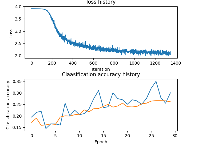
可以看到loss下降很慢,而且train_acc和var_acc中间几乎没有空隙,说明model has low capacity,我们应该增大样本容量,但同时仍要注意过拟合的问题
4.调整超参数
best_net=None #store the best model into this
#################################################################################
# TODO: Tune hyperparameters using the validation set. Store your best trained  #
# model in best_net.                                                            #
#                                                                               #
# To help debug your network, it may help to use visualizations similar to the  #
# ones we used above; these visualizations will have significant qualitative    #
# differences from the ones we saw above for the poorly tuned network.          #
#                                                                               #
# Tweaking hyperparameters by hand can be fun, but you might find it useful to  #
# write code to sweep through possible combinations of hyperparameters          #
# automatically like we did on the previous exercises.                          #
#################################################################################
learning_rate=[3e-4,1e-2,3e-1]
hidden_size=[30,50,100]
train_epoch=[30,50]
reg=[0.1,3,10]
best_val_acc=-1
best={}
for each_lr in learning_rate:
    for each_hid in hidden_size:
        for each_epo in train_epoch:
            for each_reg in reg:
                net=TwoLayerNet(input_size,each_hid,num_classes)
                stats=net.train(X_train,y_train,X_val,y_val,learning_rate=each_lr,reg=each_reg,num_epochs=each_epo)
                train_acc=stats['train_acc_history'][-1]
                val_acc=stats['val_acc_history'][-1]
                if val_acc>best_val_acc:
                    best_val_acc=val_acc
                    best_net=net
                    best['learning_rate']=each_lr
                    best['hidden_size']=each_hid
                    best['epoch']=each_epo
                    best['reg']=each_reg

for each_key in best:
    print('best net:\n '+each_key+':%e'%best[each_key])

print('best validation accuracy: %f' %best_val_acc)


 432
432

 被折叠的 条评论
为什么被折叠?
被折叠的 条评论
为什么被折叠?
 到【灌水乐园】发言


