Solving the Problem of Overfitting

Solving the Problem of Overfitting

The problem of overfitting

• Underfitting, high bias

• overfitting, high variance:

  If we have too many features, the learned hypothesis may fit the training set very well, but fail to generalize to new examples.

Debugging and Diagnosing

• address overfitting

  -plotting hypothesis（always unpractical with too many features)

  • Options:

    1. Reduce number of features

       -Manually select which features to keep.

       -Model selection algorithm(模型选择算法)

    2. Regularization

       -Keep all the features, but reduce the magnitude/values of parameters ${\theta }_j$.

       -Works well when we have a lot of features, each of which contributes a bit to predicting $y$.

Cost function

Regularization

Small values for parameters ${\theta }_0,{\theta }_1,...,{\theta }_n$

​ -“Simpler” hypothesis

​ -Less prone to overfitting

If have overfitting, we can reduce the weight that some of the items in function carry by increasing their cost.

e.g.

Want to make the following function more quadratic:

​ ${\theta }_0+{\theta }_{1}x+{\theta }_2{x}^2+{\theta }_3{x}^3+{\theta }_4{x}^4$

And we want to eliminate the influence of ${\theta }_3{x}^3$ and ${\theta }_4{x}^4$

We can modify cost function:

​ $mi{n}_{\theta }\frac{1}{2m}{\sum }_{i=1}^m(h_{\theta }(x^{(i)})-y^{(i)}{)}^2+1000\cdot {\theta }_3^2+1000\cdot {\theta }_4^2$

Added two extra terms at the end to inflate the cost of ${\theta }_3$ and ${\theta }_4$ without actually getting rid of them.

In order for the cost function get close to zero($\theta_3,\theta_4\approx$0), we will have reduce the value of ${\theta }_3$ and ${\theta }_4$ to near zero and in return greatly reduce the values of ${\theta }_3{x}^3$ and ${\theta }_4{x}^4$.

---

We could regularize all of our theta parameters in :

​ $mi{n}_{\theta }\frac{1}{2m}{\sum }_{i=1}^m(h_{\theta }(x^{(i)})-y^{(i)}{)}^2+\lambda {\sum }_{j=1}^n{\theta }_j^2$

---

$\lambda$ , the regularization parameter, determines how much the costs of parameters are inflated.

If $\lambda$ is chosen to be too large, it may smooth out the function too much and cause underfitting.

Regularized Linear Regression

Gradient Descent

${\theta }_j:={\theta }_j(1-\alpha \frac{\lambda }{m})-\alpha \frac{1}{m}{\sum }_{i=1}^m(h_{\theta }(x^{(i)}-y(i))x_j^{(i)}$

$(1-\alpha \frac{\lambda }{m})$ is always be less than 1.

Normal Equation

If $\lambda \ge 0$

$\theta =(X^{T}X+\lambda \cdot L{)}^{-1}{X}^{T}y$

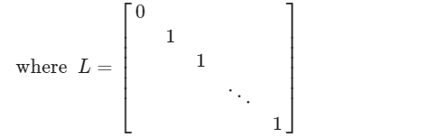
Dimension (n+1)×(n+1)

(m:#examples; n:#features)

If m < n, then $X^{T}X$ is non-invertible (singular). However, when we add the term λ⋅L, then $X^{T}X+\lambda \cdot L$ becomes invertible.

Regularized Logistic Regression

​ Cost Function

Cost function for logistic regression:

​ $J(\theta )=-\frac{1}{m}{\sum }_{i=1}^m[y^{(i)}log(h_{\theta }(x^{(i)}))+(1-y^{(i)})log(1-h_{\theta }(x^{(i)}))]$

Regularize this equation by adding a term to the end: $J(\theta )=-\frac{1}{m}{\sum }_{i=1}^m[y^{(i)}log(h_{\theta }(x^{(i)}))+(1-y^{(i)})log(1-h_{\theta }(x^{(i)}))]+\frac{\lambda }{2m}{\sum }_{j=1}^n{\theta }_j^2$

${\sum }_{j=1}^n{\theta }_j^2$ means to explicitly exclude the bias term.

da}{2m}\sum^{n_{j=1}{\theta}2_j}$

${\sum }_{j=1}^n{\theta }_j^2$ means to explicitly exclude the bias term.