


sklearn.metrics.roc_curve()
首先,需要使用sklearn.metrics.roc_curve()函数
sklearn.metrics.roc_curve(y_true, y_score, pos_label=None, sample_weight=None, drop_intermediate=True)
参数:
y_true : 数组,shape = [样本数]
在范围{0,1}或{-1,1}中真正的二进制标签。如果标签不是二进制的(多分类)则应该显式地给出pos_label
y_score : 数组, shape = [样本数]
目标得分,可以是积极类的概率估计(model.predict_proba(testdata)[:,1]),信心值,或者是决定的非阈值度量(在某些分类器上由“decision_function”返回)。
pos_label:int or str, 标签被认为是积极的,其他的被认为是消极的。
sample_weight: 顾名思义,样本的权重,可选择的
drop_intermediate: boolean, optional (default=True)
是否放弃一些不出现在绘制的ROC曲线上的次优阈值。这有助于创建更轻的ROC曲线
返回值:
注意:返回的三个数组的长度与y_score不同,具体长度怎么控制目前俺还没整明白。
fpr : array, shape = [>2]
根据thresholds与y_score得到的fpr数组
tpr : array, shape = [>2]
根据thresholds与y_score得到的tpr数组
thresholds : array, shape = [n_thresholds] ,选择的阈值数组,按照降序排列。
多分类标签须知:
使用函数label_binarize()得到的标签是一个n✖m的矩阵,n是样本的个数,m是标签类别个数。
比如三分类:
y = label_binarize(y, classes=[0, 1, 2])
array([[1, 0, 0],
       [0, 1, 0],
       [1, 0, 0],
       [0, 1, 0],
       [0, 0, 1]])
表示第1,3个样本为第一类,第2,4个样本为第二类,第5个样本为第三类。
多分类 FPR TPR 计算:
下图是多分类的混淆矩阵

TP:真正例
FP:假正例
FN:假反例
TN:真反例
对于某一类,TP只是对角线上的一块儿,FN是该类别行上除了对角线元素的部分,FP是该类别列上除了对角线元素的部分,TN是其余的部分,只要是其他类的,不管在不在该类的行和列上,都是TN。
import numpy as np
from sklearn.metrics import confusion_matrix

y_true = [1, -1,  0,  0,  1, -1,  1,  0, -1,  0,  1, -1,  1,  0,  0, -1,  0]
y_prediction = [-1, -1,  1,  0,  0,  0,  0, -1,  1, -1,  1,  1,  0,  0,  1,  1, -1]
cnf_matrix = confusion_matrix(y_true, y_prediction)
print(cnf_matrix)
#[[1 1 3]
# [3 2 2]
# [1 3 1]]

FP = cnf_matrix.sum(axis=0) - np.diag(cnf_matrix)
FN = cnf_matrix.sum(axis=1) - np.diag(cnf_matrix)
TP = np.diag(cnf_matrix)
TN = cnf_matrix.sum() - (FP + FN + TP)

FP = FP.astype(float)
FN = FN.astype(float)
TP = TP.astype(float)
TN = TN.astype(float)

# Sensitivity, hit rate, recall, or true positive rate
TPR = TP/(TP+FN)
# Specificity or true negative rate
TNR = TN/(TN+FP)
# Precision or positive predictive value
PPV = TP/(TP+FP)
# Negative predictive value
NPV = TN/(TN+FN)
# Fall out or false positive rate
FPR = FP/(FP+TN)
# False negative rate
FNR = FN/(TP+FN)
# False discovery rate
FDR = FP/(TP+FP)
# Overall accuracy
ACC = (TP+TN)/(TP+FP+FN+TN)
**例子:**
**导包:**

```python
import pyupset as pyu
from pickle import load
import os
os.chdir('D:\\train')
import numpy as np
import matplotlib.pyplot as plt
from itertools import cycle

from sklearn import svm, datasets
from sklearn.metrics import roc_curve, auc
from sklearn.model_selection import train_test_split
from sklearn.preprocessing import label_binarize
from sklearn.multiclass import OneVsRestClassifier
from scipy import interp
导数据:
iris = datasets.load_iris()
X = iris.data
y = iris.target

# Binarize the output
y = label_binarize(y, classes=[0, 1, 2])
n_classes = y.shape[1]
建立模型
# Add noisy features to make the problem harder
random_state = np.random.RandomState(0)
n_samples, n_features = X.shape
X = np.c_[X, random_state.randn(n_samples, 200 * n_features)]

# shuffle and split training and test sets
X_train, X_test, y_train, y_test = train_test_split(X, y, test_size=.5,
                                                    random_state=0)

# Learn to predict each class against the other
classifier = OneVsRestClassifier(svm.SVC(kernel='linear', probability=True,
                                 random_state=random_state))
y_score = classifier.fit(X_train, y_train).decision_function(X_test)
重点: 计算每个样本的ROC
# Compute ROC curve and ROC area for each class
fpr = dict()
tpr = dict()
roc_auc = dict()
for i in range(n_classes):
    fpr[i], tpr[i], _ = roc_curve(y_test[:, i], y_score[:, i])
    roc_auc[i] = auc(fpr[i], tpr[i])

# Compute micro-average ROC curve and ROC area
fpr["micro"], tpr["micro"], _ = roc_curve(y_test.ravel(), y_score.ravel())
roc_auc["micro"] = auc(fpr["micro"], tpr["micro"])
画图:
# Compute macro-average ROC curve and ROC area
# First aggregate all false positive rates
all_fpr = np.unique(np.concatenate([fpr[i] for i in range(n_classes)]))
# Then interpolate all ROC curves at this points
mean_tpr = np.zeros_like(all_fpr)
for i in range(n_classes):
mean_tpr += interp(all_fpr, fpr[i], tpr[i])
# Finally average it and compute AUC
mean_tpr /= n_classes
fpr["macro"] = all_fpr
tpr["macro"] = mean_tpr
roc_auc["macro"] = auc(fpr["macro"], tpr["macro"])
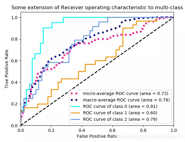
# Plot all ROC curves
plt.figure()
plt.plot(fpr["micro"], tpr["micro"],
label='micro-average ROC curve (area = {0:0.2f})'
''.format(roc_auc["micro"]),
color='deeppink', linestyle=':', linewidth=4)
plt.plot(fpr["macro"], tpr["macro"],
label='macro-average ROC curve (area = {0:0.2f})'
''.format(roc_auc["macro"]),
color='navy', linestyle=':', linewidth=4)
colors = cycle(['aqua', 'darkorange', 'cornflowerblue'])
for i, color in zip(range(n_classes), colors):
plt.plot(fpr[i], tpr[i], color=color, lw=lw,
label='ROC curve of class {0} (area = {1:0.2f})'
''.format(i, roc_auc[i]))
plt.plot([0, 1], [0, 1], 'k--', lw=lw)
plt.xlim([0.0, 1.0])
plt.ylim([0.0, 1.05])
plt.xlabel('False Positive Rate')
plt.ylabel('True Positive Rate')
plt.title('Some extension of Receiver operating characteristic to multi-class')
plt.legend(loc="lower right")
plt.show()


 8188
8188


 被折叠的 条评论
为什么被折叠?
被折叠的 条评论
为什么被折叠?
 到【灌水乐园】发言


