


Improve NN
文章目录
train/dev/test set
0.7/0/0.3 0.6.0.2.0.2 -> 100-10000
0.98/0.01/0.01 … -> big data
Bias/Variance
偏差度量的是单个模型的学习能力,而方差度量的是同一个模型在不同数据集上的稳定性。
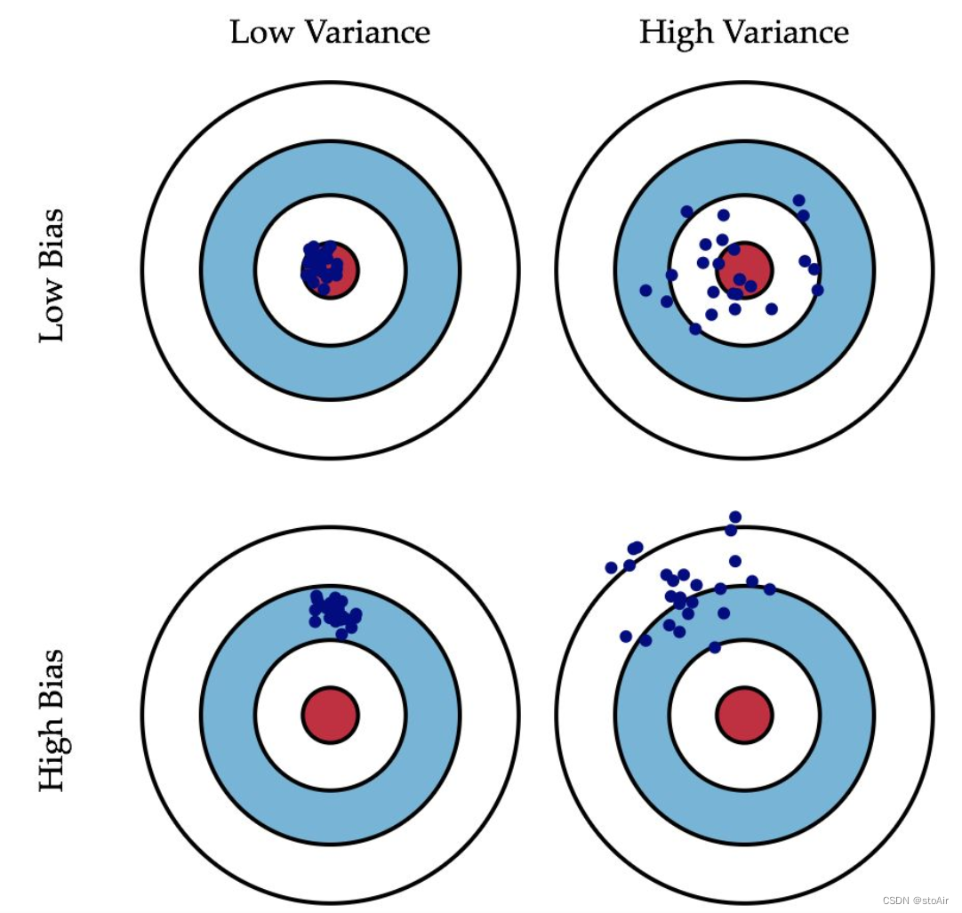
high variance ->high dev set error
high bias ->high train set error
basic recipe
high bias -> bigger network / train longer / more advanced optimization algorithms / NN architectures
high variance -> more data / regularization / NN architecture
Regularization
Logistic Regression
L 2 r e g u l a r i z a t i o n : m i n J ( w , b ) → J ( w , b ) = 1 m ∑ i = 1 m L ( y ^ ( i ) , y ( i ) ) + λ 2 m ∥ w ∥ 2 2 L2\;\; regularization:\\min\mathcal{J}(w,b)\rightarrow J(w,b)=\frac{1}{m}\sum_{i=1}^m\mathcal{L}(\hat y^{(i)},y^{(i)})+\frac{\lambda}{2m}\Vert w\Vert_2^2 L2regularization:minJ(w,b)→J(w,b)=m1i=1∑mL(y^(i),y(i))+2mλ∥w∥22
Neural network
F r o b e n i u s n o r m ∥ w [ l ] ∥ F 2 = ∑ i = 1 n [ l ] ∑ j = 1 n [ l − 1 ] ( w i , j [ l ] ) 2 D r o p o u t r e g u l a r i z a t i o n : d 3 = n p . r a n d m . r a n d ( a 3. s h a p e . s h a p e [ 0 ] , a 3. s h a p e [ 1 ] < k e e p . p r o b ) a 3 = n p . m u l t i p l y ( a 3 , d 3 ) a 3 / = k e e p . p r o b Frobenius\;\; norm\\ \Vert w^{[l]}\Vert^2_F=\sum_{i=1}^{n^{[l]}}\sum_{j=1}^{n^{[l-1]}}(w_{i,j}^{[l]})^2\\\\ Dropout\;\; regularization:\\ d3=np.randm.rand(a3.shape.shape[0],a3.shape[1]<keep.prob)\\ a3=np.multiply(a3,d3)\\ a3/=keep.prob Frobeniusnorm∥w[l]∥F2=i=1∑n[l]j=1∑n[l−1](wi,j[l])2Dropoutregularization:d3=np.randm.rand(a3.shape.shape[0],a3.shape[1]<keep.prob)a3=np.multiply(a3,d3)a3/=keep.prob
other ways
- early stopping
- data augmentation
optimization problem
speed up the training of your neural network
Normalizing inputs
- subtract mean
μ = 1 m ∑ i = 1 m x ( i ) x : = x − μ \mu =\frac{1}{m}\sum _{i=1}^{m}x^{(i)}\\ x:=x-\mu μ=m1i=1∑mx(i)x:=x−μ
- normalize variance
σ 2 = 1 m ∑ i = 1 m ( x ( i ) ) 2 x / = σ \sigma ^2=\frac{1}{m}\sum_{i=1}^m(x^{(i)})^2\\ x/=\sigma σ2=m1i=1∑m(x(i))2x/=σ
vanishing/exploding gradients
y = w [ l ] w [ l − 1 ] . . . w [ 2 ] w [ 1 ] x w [ l ] > I → ( w [ l ] ) L → ∞ w [ l ] < I → ( w [ l ] ) L → 0 y=w^{[l]}w^{[l-1]}...w^{[2]}w^{[1]}x\\ w^{[l]}>I\rightarrow (w^{[l]})^L\rightarrow\infty \\w^{[l]}<I\rightarrow (w^{[l]})^L\rightarrow0 y=w[l]w[l−1]...w[2]w[1]xw[l]>I→(w[l])L→∞w[l]<I→(w[l])L→0
weight initialize
v a r ( w ) = 1 n ( l − 1 ) w [ l ] = n p . r a n d o m . r a n d n ( s h a p e ) ∗ n p . s q r t ( 1 n ( l − 1 ) ) var(w)=\frac{1}{n^{(l-1)}}\\ w^{[l]}=np.random.randn(shape)*np.sqrt(\frac{1}{n^{(l-1)}}) var(w)=n(l−1)1w[l]=np.random.randn(shape)∗np.sqrt(n(l−1)1)
gradient check
Numerical approximation
f ( θ ) = θ 3 f ′ ( θ ) = f ( θ + ε ) − f ( θ − ε ) 2 ε f(\theta)=\theta^3\\ f'(\theta)=\frac{f(\theta+\varepsilon)-f(\theta-\varepsilon)}{2\varepsilon} f(θ)=θ3f′(θ)=2εf(θ+ε)−f(θ−ε)
grad check
d θ a p p r o x [ i ] = J ( θ 1 , . . . θ i + ε . . . ) − J ( θ 1 , . . . θ i − ε . . . ) 2 ε = d θ [ i ] c h e c k : ∥ d θ a p p r o x − d θ ∥ 2 ∥ d θ a p p r o x ∥ 2 + ∥ d θ ∥ 2 < 1 0 − 7 d\theta_{approx}[i]=\frac{J(\theta_1,...\theta_i+\varepsilon...)-J(\theta_1,...\theta_i-\varepsilon...)}{2\varepsilon}=d\theta[i]\\ check:\frac{\Vert d\theta_{approx}-d\theta\Vert_2}{\Vert d\theta_{approx}\Vert_2+\Vert d\theta\Vert_2}<10^{-7} dθapprox[i]=2εJ(θ1,...θi+ε...)−J(θ1,...θi−ε...)=dθ[i]check:∥dθapprox∥2+∥dθ∥2∥dθapprox−dθ∥2<10−7


 9358
9358


 被折叠的 条评论
为什么被折叠?
被折叠的 条评论
为什么被折叠?
 到【灌水乐园】发言


