


✅博主简介:热爱科研的Matlab仿真开发者,修心和技术同步精进,Matlab项目合作可私信。
🍎个人主页:海神之光
🏆代码获取方式:
海神之光Matlab王者学习之路—代码获取方式
⛳️座右铭:行百里者,半于九十。
更多Matlab仿真内容点击👇
Matlab图像处理(进阶版)
路径规划(Matlab)
神经网络预测与分类(Matlab)
优化求解(Matlab)
语音处理(Matlab)
信号处理(Matlab)
车间调度(Matlab)
⛄一、硬币图像识别简介
本设计为硬币图像识别统计装置,通过数码相机获取平铺无重叠堆积的硬币的图像,并通过Matlab工具处理后统计硬币的数目。
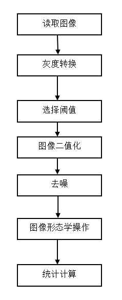
1 图像格式转换
取的图像格式为RGB彩色图像,需要先将其转换为8位256级的灰度图像。本程序采用Matlab的图像处理工具箱的函数rgb2gray来实现。
rgb2gray()
功能:
转换RGB图像或颜色映像表为灰度图像。
语法:
I = rgb2gray(RGB)
newmap = rgb2gray(map)
2 去噪及特征提取
上图1-1为硬币统计的局部图片,图中可见,硬币主体部分和背景以及图像有着明显的区别,可以通过选取合适的阈值进行二值化,从而提取出硬币的特征。
图1-2为此图像的直方图,从图中可见到比较明显的阈值分界点,但是并不是非常的明显,这是因为,图中有很多的硬币因为反光的缘故,导致主体部分有些发白,如图1-3所示。
3 灰度调整
对于这些发白部分,我们采用灰度调整及中值滤波进行处理,在matlab中,提供了两个函数进行相应的操作,其中imadjust进行灰度调整,其用法如下
Imadjst(f,[low_in high_in],[low_out high_out],gamma)
Gamma所表示的意义:
1 -------- 凹曲线
<1 -------- 凸直线
=1 -------- 直线
medfilt2用于进行中值滤波处理,其用法如下
F=medfilt2(f,[m n]);
f为输入图像
[m n]为中值滤波模板
F是中值滤波后输出的图像。
图4-1经过灰度调整及中值滤波后的图像如图1-4所示,可见,经过中值滤波后,硬币的主体部分有了较大的改善。
4 二值化处理
经过滤波后,即可对图像进行二值化处理,首先,我们采用人工选择阈值的方法进行二值化,由图可见,对于本幅图片,其合适的阈值在50~100之间,通过试验,我们选取的值为80。
对图像二值化处理的程序如下:
[M,N]=size(F);
for x=1:M
for y=1:N
if F(x,y)<80
F(x,y)=0; %低于阈值的值黑
else
F(x,y)=255; %高于阈值的值白
end
end
end
5 阈值分割
当然仍有许多模糊的硬币管脚残影,但已经将硬币的主体很好的识别了出来,采用人工选择阈值的方法虽然可以成功分离出硬币的主体,但是这个阈值这是针对这张图片有效,对于获取的其它图片,这个阈值并不能正确地对图像进行二值化处理,因此我们决定采用自动阈值分割的方法来对图像进行二值化。
我们所选用的自动阈值分割方法为Otsu法,它是一种使类间方差最大的自动确定阈值的方法,该方法具有简单、处理速度快的特点,是一种常用的阈值选取方法。
在matlab中,提供了一个函数graythresh来实现Otsu法阈值分割,其用法如下:
T=graythresh(f);
其中,f为待进行阈值分割的灰度图像,T为返回的分割灰度比例,将其乘于256即为Otsu法划定的分割阈值。
优化后的程序如下:
T=graythresh(F);
由图中可见,噪声被有效的滤除了,但是,去除了噪声的同时,也使部分接触紧密的硬币在闭运算后可能连成一个整体,如图1-8中的红圈所示,因此在此后的识别统计中需要对其进行特殊的处理。
⛄二、部分源代码
% function BlobsDemo()
% echo on;
% Startup code.
tic; % Start timer.
clc; % Clear command window.
clearvars; % Get rid of variables from prior run of this m-file.
fprintf(‘Running BlobsDemo.m…\n’); % Message sent to command window.
workspace; % Make sure the workspace panel with all the variables is showing.
imtool close all; % Close all imtool figures.
format long g;
format compact;
captionFontSize = 14;
% Check that user has the Image Processing Toolbox installed.
hasIPT = license(‘test’, ‘image_toolbox’);
if ~hasIPT
% User does not have the toolbox installed.
message = sprintf(‘Sorry, but you do not seem to have the Image Processing Toolbox.\nDo you want to try to continue anyway?’);
reply = questdlg(message, ‘Toolbox missing’, ‘Yes’, ‘No’, ‘Yes’);
if strcmpi(reply, ‘No’)
% User said No, so exit.
return;
end
end
% Read in a standard MATLAB demo image of coins (US nickles and dimes, which are 5 cent and 10 cent coins)
baseFileName = ‘coins.png’;
folder = fileparts(which(baseFileName)); % Determine where demo folder is (works with all versions).
fullFileName = fullfile(folder, baseFileName);
if ~exist(fullFileName, ‘file’)
% It doesn’t exist in the current folder.
% Look on the search path.
if ~exist(baseFileName, ‘file’)
% It doesn’t exist on the search path either.
% Alert user that we can’t find the image.
warningMessage = sprintf(‘Error: the input image file\n%s\nwas not found.\nClick OK to exit the demo.’, fullFileName);
uiwait(warndlg(warningMessage));
fprintf(1, ‘Finished running BlobsDemo.m.\n’);
return;
end
% Found it on the search path. Construct the file name.
fullFileName = baseFileName; % Note: don’t prepend the folder.
end
% If we get here, we should have found the image file.
originalImage = imread(fullFileName);
% Check to make sure that it is grayscale, just in case the user substituted their own image.
[rows, columns, numberOfColorChannels] = size(originalImage);
if numberOfColorChannels > 1
promptMessage = sprintf(‘Your image file has %d color channels.\nThis demo was designed for grayscale images.\nDo you want me to convert it to grayscale for you so you can continue?’, numberOfColorChannels);
button = questdlg(promptMessage, ‘Continue’, ‘Convert and Continue’, ‘Cancel’, ‘Convert and Continue’);
if strcmp(button, ‘Cancel’)
fprintf(1, ‘Finished running BlobsDemo.m.\n’);
return;
end
% Do the conversion using standard book formula
originalImage = rgb2gray(originalImage);
end
% Display the grayscale image.
subplot(3, 3, 1);
imshow(originalImage);
% Maximize the figure window.
set(gcf, ‘units’,‘normalized’,‘outerposition’,[0 0 1 1]);
% Force it to display RIGHT NOW (otherwise it might not display until it’s all done, unless you’ve stopped at a breakpoint.)
drawnow;
caption = sprintf(‘Original “coins” image showing\n6 nickels (the larger coins) and 4 dimes (the smaller coins).’);
title(caption, ‘FontSize’, captionFontSize);
axis image; % Make sure image is not artificially stretched because of screen’s aspect ratio.
% Just for fun, let’s get its histogram and display it.
[pixelCount, grayLevels] = imhist(originalImage);
subplot(3, 3, 2);
bar(pixelCount);
title(‘Histogram of original image’, ‘FontSize’, captionFontSize);
xlim([0 grayLevels(end)]); % Scale x axis manually.
grid on;
% Threshold the image to get a binary image (only 0’s and 1’s) of class “logical.”
% Method #1: using im2bw()
% normalizedThresholdValue = 0.4; % In range 0 to 1.
% thresholdValue = normalizedThresholdValue * max(max(originalImage)); % Gray Levels.
% binaryImage = im2bw(originalImage, normalizedThresholdValue); % One way to threshold to binary
% Method #2: using a logical operation.
thresholdValue = 100;
binaryImage = originalImage > thresholdValue; % Bright objects will be chosen if you use >.
% ========== IMPORTANT OPTION ============================================================
% Use < if you want to find dark objects instead of bright objects.
% binaryImage = originalImage < thresholdValue; % Dark objects will be chosen if you use <.
% Do a “hole fill” to get rid of any background pixels or “holes” inside the blobs.
binaryImage = imfill(binaryImage, ‘holes’);
% Show the threshold as a vertical red bar on the histogram.
hold on;
maxYValue = ylim;
line([thresholdValue, thresholdValue], maxYValue, ‘Color’, ‘r’);
% Place a text label on the bar chart showing the threshold.
annotationText = sprintf(‘Thresholded at %d gray levels’, thresholdValue);
% For text(), the x and y need to be of the data class “double” so let’s cast both to double.
text(double(thresholdValue + 5), double(0.5 * maxYValue(2)), annotationText, ‘FontSize’, 10, ‘Color’, [0 .5 0]);
text(double(thresholdValue - 70), double(0.94 * maxYValue(2)), ‘Background’, ‘FontSize’, 10, ‘Color’, [0 0 .5]);
text(double(thresholdValue + 50), double(0.94 * maxYValue(2)), ‘Foreground’, ‘FontSize’, 10, ‘Color’, [0 0 .5]);
% Display the binary image.
subplot(3, 3, 3);
imshow(binaryImage);
title(‘Binary Image, obtained by thresholding’, ‘FontSize’, captionFontSize);
% Identify individual blobs by seeing which pixels are connected to each other.
% Each group of connected pixels will be given a label, a number, to identify it and distinguish it from the other blobs.
% Do connected components labeling with either bwlabel() or bwconncomp().
labeledImage = bwlabel(binaryImage, 8); % Label each blob so we can make measurements of it
% labeledImage is an integer-valued image where all pixels in the blobs have values of 1, or 2, or 3, or … etc.
subplot(3, 3, 4);
imshow(labeledImage, []); % Show the gray scale image.
title(‘Labeled Image, from bwlabel()’, ‘FontSize’, captionFontSize);
% Let’s assign each blob a different color to visually show the user the distinct blobs.
coloredLabels = label2rgb (labeledImage, ‘hsv’, ‘k’, ‘shuffle’); % pseudo random color labels
% coloredLabels is an RGB image. We could have applied a colormap instead (but only with R2014b and later)
subplot(3, 3, 5);
imshow(coloredLabels);
axis image; % Make sure image is not artificially stretched because of screen’s aspect ratio.
caption = sprintf(‘Pseudo colored labels, from label2rgb().\nBlobs are numbered from top to bottom, then from left to right.’);
title(caption, ‘FontSize’, captionFontSize);
% Get all the blob properties. Can only pass in originalImage in version R2008a and later.
blobMeasurements = regionprops(labeledImage, originalImage, ‘all’);
numberOfBlobs = size(blobMeasurements, 1);
% bwboundaries() returns a cell array, where each cell contains the row/column coordinates for an object in the image.
% Plot the borders of all the coins on the original grayscale image using the coordinates returned by bwboundaries.
subplot(3, 3, 6);
imshow(originalImage);
title(‘Outlines, from bwboundaries()’, ‘FontSize’, captionFontSize);
axis image; % Make sure image is not artificially stretched because of screen’s aspect ratio.
hold on;
boundaries = bwboundaries(binaryImage);
numberOfBoundaries = size(boundaries, 1);
for k = 1 : numberOfBoundaries
thisBoundary = boundaries{k};
plot(thisBoundary(:,2), thisBoundary(:,1), ‘g’, ‘LineWidth’, 2);
end
hold off;
textFontSize = 14; % Used to control size of “blob number” labels put atop the image.
labelShiftX = -7; % Used to align the labels in the centers of the coins.
blobECD = zeros(1, numberOfBlobs);
% Print header line in the command window.
fprintf(1,‘Blob # Mean Intensity Area Perimeter Centroid Diameter\n’);
% Loop over all blobs printing their measurements to the command window.
for k = 1 : numberOfBlobs % Loop through all blobs.
% Find the mean of each blob. (R2008a has a better way where you can pass the original image
% directly into regionprops. The way below works for all versions including earlier versions.)
thisBlobsPixels = blobMeasurements(k).PixelIdxList; % Get list of pixels in current blob.
meanGL = mean(originalImage(thisBlobsPixels)); % Find mean intensity (in original image!)
meanGL2008a = blobMeasurements(k).MeanIntensity; % Mean again, but only for version >= R2008a
blobArea = blobMeasurements(k).Area;		% Get area.
blobPerimeter = blobMeasurements(k).Perimeter;		% Get perimeter.
blobCentroid = blobMeasurements(k).Centroid;		% Get centroid one at a time
blobECD(k) = sqrt(4 * blobArea / pi);					% Compute ECD - Equivalent Circular Diameter.
fprintf(1,'#%2d %17.1f %11.1f %8.1f %8.1f %8.1f % 8.1f\n', k, meanGL, blobArea, blobPerimeter, blobCentroid, blobECD(k));
% Put the "blob number" labels on the "boundaries" grayscale image.
text(blobCentroid(1) + labelShiftX, blobCentroid(2), num2str(k), 'FontSize', textFontSize, 'FontWeight', 'Bold');
end
% Now, I’ll show you another way to get centroids.
% We can get the centroids of ALL the blobs into 2 arrays,
% one for the centroid x values and one for the centroid y values.
allBlobCentroids = [blobMeasurements.Centroid];
centroidsX = allBlobCentroids(1:2:end-1);
centroidsY = allBlobCentroids(2:2:end);
% Put the labels on the rgb labeled image also.
subplot(3, 3, 5);
for k = 1 : numberOfBlobs % Loop through all blobs.
text(centroidsX(k) + labelShiftX, centroidsY(k), num2str(k), ‘FontSize’, textFontSize, ‘FontWeight’, ‘Bold’);
end
% Now I’ll demonstrate how to select certain blobs based using the ismember() function.
% Let’s say that we wanted to find only those blobs
% with an intensity between 150 and 220 and an area less than 2000 pixels.
% This would give us the three brightest dimes (the smaller coin type).
allBlobIntensities = [blobMeasurements.MeanIntensity];
allBlobAreas = [blobMeasurements.Area];
% Get a list of the blobs that meet our criteria and we need to keep.
% These will be logical indices - lists of true or false depending on whether the feature meets the criteria or not.
% for example [1, 0, 0, 1, 1, 0, 1, …]. Elements 1, 4, 5, 7, … are true, others are false.
allowableIntensityIndexes = (allBlobIntensities > 150) & (allBlobIntensities < 220);
allowableAreaIndexes = allBlobAreas < 2000; % Take the small objects.
% Now let’s get actual indexes, rather than logical indexes, of the features that meet the criteria.
% for example [1, 4, 5, 7, …] to continue using the example from above.
keeperIndexes = find(allowableIntensityIndexes & allowableAreaIndexes);
% Extract only those blobs that meet our criteria, and
% eliminate those blobs that don’t meet our criteria.
% Note how we use ismember() to do this. Result will be an image - the same as labeledImage but with only the blobs listed in keeperIndexes in it.
keeperBlobsImage = ismember(labeledImage, keeperIndexes);
% Re-label with only the keeper blobs kept.
labeledDimeImage = bwlabel(keeperBlobsImage, 8); % Label each blob so we can make measurements of it
% Now we’re done. We have a labeled image of blobs that meet our specified criteria.
subplot(3, 3, 7);
imshow(labeledDimeImage, []);
axis image;
title(‘“Keeper” blobs (3 brightest dimes in a re-labeled image)’, ‘FontSize’, captionFontSize);
% Plot the centroids in the original image in the upper left.
% Dimes will have a red cross, nickels will have a blue X.
message = sprintf(‘Now I will plot the centroids over the original image in the upper left.\nPlease look at the upper left image.’);
reply = questdlg(message, ‘Plot Centroids?’, ‘OK’, ‘Cancel’, ‘Cancel’);
% Note: reply will = ‘’ for Upper right X, ‘OK’ for OK, and ‘Cancel’ for Cancel.
if strcmpi(reply, ‘Cancel’)
return;
end
subplot(3, 3, 1);
hold on; % Don’t blow away image.
for k = 1 : numberOfBlobs % Loop through all keeper blobs.
% Identify if blob #k is a dime or nickel.
itsADime = allBlobAreas(k) < 2200; % Dimes are small.
if itsADime
% Plot dimes with a red +.
plot(centroidsX(k), centroidsY(k), ‘r+’, ‘MarkerSize’, 10, ‘LineWidth’, 2);
else
% Plot dimes with a blue x.
plot(centroidsX(k), centroidsY(k), ‘bx’, ‘MarkerSize’, 10, ‘LineWidth’, 2);
end
end
⛄三、运行结果


⛄四、matlab版本及参考文献
1 matlab版本
2014a
2 参考文献
[1]朱俊达.硬币分拣机的分拣与计数[J].技术与市场. 2018,25(02)
3 备注
简介此部分摘自互联网,仅供参考,若侵权,联系删除
🍅 仿真咨询
1 各类智能优化算法改进及应用
生产调度、经济调度、装配线调度、充电优化、车间调度、发车优化、水库调度、三维装箱、物流选址、货位优化、公交排班优化、充电桩布局优化、车间布局优化、集装箱船配载优化、水泵组合优化、解医疗资源分配优化、设施布局优化、可视域基站和无人机选址优化
2 机器学习和深度学习方面
卷积神经网络(CNN)、LSTM、支持向量机(SVM)、最小二乘支持向量机(LSSVM)、极限学习机(ELM)、核极限学习机(KELM)、BP、RBF、宽度学习、DBN、RF、RBF、DELM、XGBOOST、TCN实现风电预测、光伏预测、电池寿命预测、辐射源识别、交通流预测、负荷预测、股价预测、PM2.5浓度预测、电池健康状态预测、水体光学参数反演、NLOS信号识别、地铁停车精准预测、变压器故障诊断
3 图像处理方面
图像识别、图像分割、图像检测、图像隐藏、图像配准、图像拼接、图像融合、图像增强、图像压缩感知
4 路径规划方面
旅行商问题(TSP)、车辆路径问题(VRP、MVRP、CVRP、VRPTW等)、无人机三维路径规划、无人机协同、无人机编队、机器人路径规划、栅格地图路径规划、多式联运运输问题、车辆协同无人机路径规划、天线线性阵列分布优化、车间布局优化
5 无人机应用方面
无人机路径规划、无人机控制、无人机编队、无人机协同、无人机任务分配
6 无线传感器定位及布局方面
传感器部署优化、通信协议优化、路由优化、目标定位优化、Dv-Hop定位优化、Leach协议优化、WSN覆盖优化、组播优化、RSSI定位优化
7 信号处理方面
信号识别、信号加密、信号去噪、信号增强、雷达信号处理、信号水印嵌入提取、肌电信号、脑电信号、信号配时优化
8 电力系统方面
微电网优化、无功优化、配电网重构、储能配置
9 元胞自动机方面
交通流 人群疏散 病毒扩散 晶体生长
10 雷达方面
卡尔曼滤波跟踪、航迹关联、航迹融合


 4437
4437


 被折叠的 条评论
为什么被折叠?
被折叠的 条评论
为什么被折叠?
 到【灌水乐园】发言


