【线性回归（2）】多元线性回归（多项式线性回归）

1 概述

一元线性回归只能拟合$y=ax+b$，或者说只能拟合直线。
其实对于多元线性回归来说，$x_2,x_3...$是不同于$x_1=x$的另一个特征，方程可表示为：
$$y={\theta }_1{x}_1+{\theta }_2{x}_2+...+{\theta }_n{x}_n+{\theta }_0$$
$x_1,x_2...$是因变量（特征），${\theta }_1,{\theta }_2...$是系数，${\theta }_0$是截距。
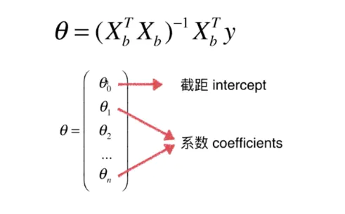
多元线性回归可以用特征方程去求解。

代码实现：

import numpy as np

class LinearRegression():
    def __init__(self):
        self._theta = None
        self.coef = None
        self.interception = None

    def fit(self, X_train, y_train):
        X_b = np.hstack([np.ones((X_train.shape[0] ,1)), X_train])

        self._theta = np.linalg.inv(X_b.T.dot(X_b)).dot(X_b.T).dot(y_train)

        self.coef = self._theta[1:]

        self.interception = self._theta[0]
        
        return self

    def predict(self, X_test):
        X_b = np.hstack([np.ones((X_test.shape[0] ,1)), X_test])
        return X_b.dot(self._theta)

2 多项式线性回归

多项式线性回归是多元线性回归中比较特殊的一类，只有一个因变量$x$，其它的特征是$x$的几次方，比如$y=a{x}^2+bx+c$或者是更高次数的方程：
$$y={\theta }_{1}x+{\theta }_2{x}^2+...+{\theta }_n{x}^n+{\theta }_0$$

以$y=a{x}^2+bx+c$为例：

import numpy as np
from matplotlib import pyplot as plt

x = np.random.uniform(-3, 3, size=100)
x = np.sort(x)
X = x.reshape(-1, 1)
# X.shape (100, 1)

y = 0.5*x**2 + x + 2 + np.random.normal(0, 1, 100)
# y.shape (100,)

plt.scatter(X, y)

这是一个抛物线，如果再用一元线性回归去拟合，就是下面的样子，可以发现误差时非常大的：

一元线性回归只有一个特征$x$，多项式回归则是添加新的特征（$x^2,x^3...$），这里我只需要添加$x$的平方，来拟合一个抛物线。

3.1 使用np.hstack函数

# 使用np.hstack函数，将两个特征在水平方向上拼接
X2 = np.hstack([X, X**2]) # 拼接
# X2.shape (100, 2)

'''
注:  np.vstack() :在竖直方向上堆叠
	 np.hstack() :在水平方向上拼接
'''

from sklearn.linear_model import LinearRegression
lin_reg = LinearRegression()
lin_reg.fit(X2, y)
y_predict = lin_reg.predict(X2)
print(lin_reg.coef_) # 系数 a, b
# array([1.04078131, 0.54484198])
print(lin_reg.intercept_) # 截距 c
# 1.9212545662064286

# 绘制一下图像
plt.scatter(X, y, color="b")
plt.plot(x, y_predict, color="r")

3.2 PolynomialFeatures

from sklearn.preprocessing import PolynomialFeatures

# 构造多项式，如果只有一个x，degree=2，则为[1, x, x^2]，其中1代表截距列
poly = PolynomialFeatures(degree=2)

poly.fit(X)

X3 = poly.transform(X) # 构建X
X3.shape  # （100，3）

同样的，用LinearRegression()拟合。

lin_reg = LinearRegression()
lin_reg.fit(X3, y)
y_predict = lin_reg.predict(X3)

3.3 pipeline

from sklearn.pipeline import  Pipeline
from sklearn.preprocessing import StandardScaler

# 三合一
poly_reg = Pipeline([
	("ploy", PolynomialFeatures(degree=2)), # 生成多项式特征
	("std_scaler", StandardScaler()),       # 数据归一化
	("lin_reg", LinearRegression())         # 进行线性回归
])

poly_reg.fit(X, y)
y_predict = poly_reg.predict(X)

plt.scatter(X, y, color="b")
plt.plot(x, y_predict, color="r")