


PyTorch 模块和基础实战
Follow Datawhale 的 《深入浅出 PyTorch》
PyTorch 模块和基础实战
PyTorch 基本模块
基本配置
导入必要的包:
import os
import numpy as np
import pandas as pd
import torch
import torch.nn as nn
import torch.optim as optim
from torch.utils.data import Dataset, DataLoader
超参数的统一设置:
- batch size;
- learning rate;
- 训练次数(max_epochs)
- GPU 设置
batch_size = 16 	# 批次的大小
lr = 1e-4			# 优化器的学习率
max_epochs = 100	# 训练次数
GPU 设置的常见方案:
# 方案一:使用os.environ,这种情况如果使用GPU不需要设置
os.environ['CUDA_VISIBLE_DEVICES'] = '0,1'

# 方案二:使用“device”,后续对要使用GPU的变量用.to(device)即可
device = torch.device("cuda:1" if torch.cuda.is_available() else "cpu")

print(device)
cuda:1
数据读入
PyTorch 数据读入是通过 Dataset+DataLoader 的方式完成的,Dataset 定义好数据的格式和数据变换形式,DataLoader 用 iterative 的方式不断读入批次数据。
我们可以定义自己的 Dataset 类来实现灵活的数据读取,定义的类需要继承 PyTorch 自身的 Dataset 类。主要包含三个函数:
__init__:用于向类中传入外部参数,同时定义样本集;__getitem__:用于逐个读取样本集合中的元素,可以进行一定的变换,并将返回训练/验证所需的数据;__len__:用于返回数据集的样本数。
这里另外给出一个例子,其中图片存放在一个文件夹,另外有一个 csv 文件给出了图片名称对应的标签。这种情况下需要自己来定义 Dataset 类:
class MyDataset(Dataset):
    def __init__(self, data_dir, info_csv, image_list, transform=None):
        """
        Args:
            data_dir: path to image directory.
            info_csv: path to the csv file containing image indexes
                with corresponding labels.
            image_list: path to the txt file contains image names to training/validation set
            transform: optional transform to be applied on a sample.
        """
        label_info = pd.read_csv(info_csv)
        image_file = open(image_list).readlines()
        self.data_dir = data_dir
        self.image_file = image_file
        self.label_info = label_info
        self.transform = transform

    def __getitem__(self, index):
        """
        Args:
            index: the index of item
        Returns:
            image and its labels
        """
        image_name = self.image_file[index].strip('\n')
        raw_label = self.label_info.loc[self.label_info['Image_index'] == image_name]
        label = raw_label.iloc[:,0]
        image_name = os.path.join(self.data_dir, image_name)
        image = Image.open(image_name).convert('RGB')
        if self.transform is not None:
            image = self.transform(image)
        return image, label

    def __len__(self):
        return len(self.image_file)
构建好 Dataset 后,就可以使用 DataLoader 来按批次读入数据了,实现代码如下:
from torch.utils.data import DataLoader

train_loader = torch.utils.data.DataLoader(train_data, batch_size=batch_size, num_workers=4, shuffle=True, drop_last=True)

val_loader = torch.utils.data.DataLoader(val_data, batch_size=batch_size, num_workers=4, shuffle=False)
其中:
batch_size:样本是按 “批” 读入的,batch_size就是每次读入的样本数;num_workers:有多少个进程用于读取数据;shuffle:是否将读入的数据打乱;drop_last:对于样本最后一部分没有达到批次数的样本,使其不再参与训练。
模型构建
PyTorch 中神经网络构造一般是基于 Module 类的模型来完成的,它让模型构造更加灵活。Module 类是 nn 模块里提供的一个模型构造类,是所有神经网络模块的基类。下面继承 Module 类构造多层感知机。
import torch
from torch import nn

class MLP(nn.Module):
  # 声明带有模型参数的层,这里声明了两个全连接层
  def __init__(self, **kwargs):
    # 调用MLP父类Block的构造函数来进行必要的初始化。这样在构造实例时还可以指定其他函数
    super(MLP, self).__init__(**kwargs)
    self.hidden = nn.Linear(784, 256)
    self.act = nn.ReLU()
    self.output = nn.Linear(256,10)

   # 定义模型的前向计算,即如何根据输入x计算返回所需要的模型输出
  def forward(self, x):
    o = self.act(self.hidden(x))
    return self.output(o)
以上的 MLP 类中无须定义反向传播函数。系统将通过自动求梯度而自动生成反向传播所需的 backward 函数。
我们可以实例化 MLP 类得到模型变量 net 。下面的代码初始化 net 并传入输入数据 X 做一次前向计算。其中, net(X) 会调用 MLP 继承自 Module 类的 call 函数,这个函数将调用 MLP 类定义的 forward 函数来完成前向计算。
X = torch.rand(2, 784)
net = MLP()
print(net)
print(net(X))
MLP(
  (hidden): Linear(in_features=784, out_features=256, bias=True)
  (act): ReLU()
  (output): Linear(in_features=256, out_features=10, bias=True)
)
tensor([[ 4.6889e-02,  5.4081e-02,  2.3431e-02,  2.9768e-01, -8.3136e-02,
         -2.9591e-02,  3.5421e-01,  1.5387e-01,  5.4498e-02,  8.1761e-02],
        [ 2.4696e-02,  1.0500e-01, -7.4457e-02,  3.1346e-01, -1.0509e-02,
          6.1309e-02,  3.6088e-01,  3.2176e-04, -1.1483e-02,  1.3970e-01]],
       grad_fn=<AddmmBackward0>)
模型初始化
torch.nn.init 提供了以下初始化方法:
torch.nn.init.uniform_(tensor, a=0.0, b=1.0)torch.nn.init.normal_(tensor, mean=0.0, std=1.0)torch.nn.init.constant_(tensor, val)torch.nn.init.ones_(tensor)torch.nn.init.zeros_(tensor)torch.nn.init.eye_(tensor)torch.nn.init.dirac_(tensor, groups=1)torch.nn.init.xavier_uniform_(tensor, gain=1.0)torch.nn.init.xavier_normal_(tensor, gain=1.0)torch.nn.init.kaiming_uniform_(tensor, a=0, mode='fan__in', nonlinearity='leaky_relu')torch.nn.init.kaiming_normal_(tensor, a=0, mode='fan_in', nonlinearity='leaky_relu')torch.nn.init.orthogonal_(tensor, gain=1)torch.nn.init.sparse_(tensor, sparsity, std=0.01)torch.nn.init.calculate_gain(nonlinearity, param=None)
我们可以发现这些函数除了calculate_gain,所有函数的后缀都带有下划线,意味着这些函数将会直接原地更改输入张量的值。
损失函数
二分类交叉熵损失函数
torch.nn.BCELoss(weight=None, size_average=None, reduce=None, reduction='mean')
功能:计算二分类任务时的交叉熵(Cross Entropy)函数。在二分类中,label 是 { 0 , 1 } \{0,1\} {0,1}。对于进入交叉熵函数的 i n p u t input input 为概率分布的形式。一般来说, i n p u t input input 为 s i g m o i d sigmoid sigmoid 激活层的输出,或者 s o f t m a x softmax softmax 的输出。
主要参数:
weight:每个类别的
l
o
s
s
loss
loss 设置权值;
size_average:数据为
b
o
o
l
bool
bool,为
T
r
u
e
True
True 时,返回的
l
o
s
s
loss
loss 为平均值;为
F
a
l
s
e
False
False 时,返回的各样本的
l
o
s
s
loss
loss 之和;
reduce:数据类型为
b
o
o
l
bool
bool,为
T
r
u
e
True
True 时,
l
o
s
s
loss
loss 的返回是标量。
计算公式:
l
(
x
,
y
)
=
{
m
e
a
n
(
L
)
,
if reduction=’mean’
s
u
m
(
L
)
,
if reduction=’sum’
{\mathscr l}(x,y)= \begin{cases} mean(L),&\text{if reduction='mean'}\\ sum(L),&\text{if reduction='sum'} \end{cases}
l(x,y)={mean(L),sum(L),if reduction=’mean’if reduction=’sum’
交叉熵损失函数
torch.nn.CrossEntropyLoss(weight=None, size_average=None, ignore_index=-100, reduce=None, reduction='mean')
功能:计算交叉熵函数。
主要参数:
weight:每个类别的
l
o
s
s
loss
loss 设置权值;
size_average:数据为
b
o
o
l
bool
bool,为
T
r
u
e
True
True 时,返回的
l
o
s
s
loss
loss 为平均值;为
F
a
l
s
e
False
False 时,返回的各样本的
l
o
s
s
loss
loss 之和;
ignore_index:忽略某个类的损失函数;
reduce:数据类型为
b
o
o
l
bool
bool,为
T
r
u
e
True
True 时,
l
o
s
s
loss
loss 的返回是标量。
计算公式:
loss
(
x
,
class
)
=
−
log
(
exp
x
[
class
]
∑
j
exp
(
x
[
j
]
)
)
=
−
x
[
class
]
+
log
(
∑
j
exp
(
x
[
j
]
)
)
\text{loss}(x,\text{class})=-\log\left(\frac{\exp x[\text{class}]}{\sum_j\exp(x[j])}\right)=-x[\text{class}]+\log\left(\sum_j\exp(x[j])\right)
loss(x,class)=−log(∑jexp(x[j])expx[class])=−x[class]+log(j∑exp(x[j]))
L 1 L1 L1 损失函数
torch.nn.L1Loss(size_average=None, reduce=None, reduction='mean')
功能: 计算输出 y 和真实标签 target 之间的差值的绝对值。
我们需要知道的是,reduction 参数决定了计算模式。有三种计算模式可选 —— none:逐个元素计算;sum:所有元素求和,返回标量;mean:加权平均,返回标量。 如果选择none,那么返回的结果是和输入元素相同尺寸的。默认计算方式是求平均。
计算公式如下:
L
n
=
∣
x
n
−
y
n
∣
L_n=|x_n-y_n|
Ln=∣xn−yn∣
M S E MSE MSE 损失函数
torch.nn.MSELoss(size_average=None, reduce=None, reduction='mean')
功能: 计算输出 y 和真实标签 target 之差的平方。
和 L1Loss 一样,MSELoss 损失函数中,reduction 参数决定了计算模式。有三种计算模式可选:none:逐个元素计算;sum:所有元素求和,返回标量;mean:加权平均,返回标量。默认计算方式是求平均。
计算公式如下:
l
n
=
(
x
n
−
y
n
)
2
l_n={(x_n-y_n)}^2
ln=(xn−yn)2
平滑 L 1 L1 L1 ( Smooth L1 \text{Smooth L1} Smooth L1)损失函数
torch.nn.SmoothL1Loss(size_average=None, reduce=None, reduction='mean', beta=1.0)
功能: L 1 L1 L1 的平滑输出,其功能是减轻离群点带来的影响。
reduction参数决定了计算模式。有三种计算模式可选:none:逐个元素计算;sum:所有元素求和,返回标量;mean:加权平均,返回标量。默认计算方式是求平均。
提醒: 之后的损失函数中,关于reduction 这个参数依旧会存在。所以,之后就不再单独说明。
计算公式如下:
loss
(
x
,
y
)
=
1
n
∑
i
=
1
n
z
i
,
其中
z
i
=
{
1
2
(
x
i
−
y
i
)
2
,
if
∣
x
i
−
y
i
∣
<
1
∣
x
i
−
y
i
∣
−
1
2
,
otherwise
\text{loss}(x,y)=\frac{1}{n}\sum_{i=1}^nz_i,\ 其中\ z_i= \begin{cases} \frac{1}{2}{(x_i-y_i)}^2,&\text{if}\ |x_i-y_i|<1\\ |x_i-y_i|-\frac{1}{2},&\text{otherwise} \end{cases}
loss(x,y)=n1i=1∑nzi, 其中 zi={21(xi−yi)2,∣xi−yi∣−21,if ∣xi−yi∣<1otherwise
目标泊松分布的负对数似然损失
torch.nn.PoissonNLLLoss(log_input=True, full=False, size_average=None, eps=1e-08, reduce=None, reduction='mean')
功能: 泊松分布的负对数似然损失函数。
主要参数:
log_input:输入是否为对数形式,决定计算公式;
full:计算所有
l
o
s
s
loss
loss,默认为
F
a
l
s
e
False
False;
eps:修正项,避免
i
n
p
u
t
input
input 为
0
0
0 时,
l
o
g
(
i
n
p
u
t
)
log(input)
log(input) 为
n
a
n
nan
nan 的情况。
数学公式:
- 当参数 l o g ( i n p u t ) = T r u e log(input)=True log(input)=True:
loss ( x n , y n ) = e x n − x n ⋅ y n \text{loss}(x_n,y_n)=e^{x_n}-x_n\cdot y_n loss(xn,yn)=exn−xn⋅yn
- 当参数 l o g ( i n p u t ) = F a l s e log(input)=False log(input)=False:
loss ( x n , y n ) = x n − y n ⋅ log ( x n + eps ) \text{loss}(x_n,y_n)=x_n-y_n\cdot \log(x_n+\text{eps}) loss(xn,yn)=xn−yn⋅log(xn+eps)
K L KL KL 散度
torch.nn.KLDivLoss(size_average=None, reduce=None, reduction='mean', log_target=False)
功能: 计算KL散度,也就是计算相对熵。用于连续分布的距离度量,并且对离散采用的连续输出空间分布进行回归通常很有用。
主要参数:
reduction:计算模式。可为 none:逐个元素计算;sum:所有元素求和,返回标量;mean:加权平均,返回标量;batchmean:
b
a
t
c
h
s
i
z
e
batchsize
batchsize 维度求平均值。
计算公式:
D
KL
=
E
X
∼
P
[
log
P
(
X
)
Q
(
X
)
]
=
E
X
∼
P
[
log
P
(
X
)
−
log
Q
(
X
)
]
=
∑
i
=
1
n
P
(
x
i
)
(
log
P
(
x
i
)
−
log
Q
(
x
i
)
)
\begin{align} D_{\text{KL}}={\rm E}_{X\sim P}[\log \frac{P(X)}{Q(X)}] &={\rm E}_{X\sim P}[\log P(X)-\log Q(X)]\\ &=\sum_{i=1}^n P(x_i)(\log P(x_i)-\log Q(x_i)) \end{align}
DKL=EX∼P[logQ(X)P(X)]=EX∼P[logP(X)−logQ(X)]=i=1∑nP(xi)(logP(xi)−logQ(xi))
MarginRankingLoss
torch.nn.MarginRankingLoss(margin=0.0, size_average=None, reduce=None, reduction='mean')
功能: 计算两个向量之间的相似度,用于排序任务。该方法用于计算两组数据之间的差异。
主要参数:
margin:边界值,
x
1
x_1
x1 与
x
2
x_2
x2 之间的差异值;
reduction:计算模式,可为 none/sum/mean。
计算公式:
loss
(
x
1
,
x
2
,
y
)
=
max
(
0
,
−
y
×
(
x
1
−
x
2
)
+
margin
)
\text{loss}(x_1,x_2,y)=\max(0,-y \times (x_1-x_2)+\text{margin})
loss(x1,x2,y)=max(0,−y×(x1−x2)+margin)
多标签边界损失函数
torch.nn.MultiLabelMarginLoss(size_average=None, reduce=None, reduction='mean')
功能:对于多标签分类问题计算损失函数。
主要参数:
reduction:计算模式,可为 none/sum/mean。
计算公式:
loss
(
x
,
y
)
=
∑
i
j
max
(
0
,
1
−
x
[
y
[
j
]
]
−
x
[
i
]
)
x
⋅
size
(
0
)
\text{loss}(x,y)=\sum_{ij}\frac{\max(0,1-x[y[j]]-x[i])}{x\cdot \text{size}(0)}
loss(x,y)=ij∑x⋅size(0)max(0,1−x[y[j]]−x[i])
其中,
i
=
0
,
…
,
x
⋅
size
(
0
)
,
j
=
0
,
…
,
y
⋅
size
(
0
)
i=0,\ \dots,\ x\cdot \text{size}(0),\ j=0,\ \dots,\ y\cdot \text{size}(0)
i=0, …, x⋅size(0), j=0, …, y⋅size(0),对于所有的
i
i
i 和
j
j
j,都有
y
[
j
]
≥
0
y[j]\ge0
y[j]≥0 且
i
≠
y
[
j
]
i\ne y[j]
i=y[j]。
二分类损失函数
torch.nn.SoftMarginLoss(size_average=None, reduce=None, reduction='mean')
功能:计算二分类的 l o g i s t i c logistic logistic 损失。
主要参数:
reduction:计算模式,可为 none/sum/mean。
计算公式:
loss
(
x
,
y
)
=
∑
i
log
(
1
+
exp
(
−
y
[
i
]
⋅
x
[
i
]
)
)
x
⋅
nelement
(
)
\text{loss}(x,y)=\sum_i \frac{\log(1+\exp (-y[i]\cdot x[i]))}{x \cdot \text{nelement}()}
loss(x,y)=i∑x⋅nelement()log(1+exp(−y[i]⋅x[i]))
其中,
x
⋅
nelement
(
)
x \cdot \text{nelement}()
x⋅nelement() 为输入
x
x
x 中的样本个数。注意这里的
y
y
y 也有
1
1
1 和
−
1
-1
−1 两种模式。
多分类的折页损失
torch.nn.MultiMarginLoss(p=1, margin=1.0, weight=None, size_average=None, reduce=None, reduction='mean')
功能: 计算多分类的折页损失。
主要参数:
reduction:计算模式,可为 none/sum/mean;
p:可选
1
1
1 或
2
2
2;
weight:各类别的
l
o
s
s
loss
loss 设置权值;
margin:边界值。
计算公式:
loss
(
x
,
y
)
=
∑
i
max
(
0
,
margin
−
x
[
y
]
+
x
[
i
]
)
p
x
⋅
size
(
0
)
\text{loss}(x,y)=\frac{\sum_i{\max(0,\text{margin}-x[y]+x[i])}^p}{x\cdot \text{size}(0)}
loss(x,y)=x⋅size(0)∑imax(0,margin−x[y]+x[i])p
其中,
x
∈
{
0
,
…
,
x
⋅
size
(
0
)
−
1
}
,
y
∈
{
0
,
…
,
y
⋅
size
(
0
)
−
1
}
x\in\{0,\ \dots,\ x\cdot \text{size}(0)-1\},\ y\in\{0,\ \dots,\ y\cdot \text{size}(0)-1\}
x∈{0, …, x⋅size(0)−1}, y∈{0, …, y⋅size(0)−1},并且对所有的
i
i
i 和
j
j
j,都有
0
≤
y
[
j
]
≤
x
⋅
size
(
0
)
−
1
0\le y[j]\le x\cdot \text{size}(0)-1
0≤y[j]≤x⋅size(0)−1,以及
i
≠
y
[
j
]
i\ne y[j]
i=y[j]。
三元组损失
torch.nn.TripletMarginLoss(margin=1.0, p=2.0, eps=1e-06, swap=False, size_average=None, reduce=None, reduction='mean')
功能:计算三元组损失。
三元组:这是一种数据的存储或者使用格式。<实体1,关系,实体2>。在项目中,也可以表示为< anchor, positive examples , negative examples>。
在这个损失函数中,我们希望去anchor的距离更接近positive examples,而远离negative examples。
主要参数:
reduction:计算模式,可为 none/sum/mean;
p:可选
1
1
1 或
2
2
2;
margin:边界值。
计算公式:
L
(
a
,
p
,
n
)
=
max
{
d
(
a
i
,
p
i
)
−
d
(
a
i
,
n
i
)
+
margin
,
0
}
L(a,p,n)=\max\{d(a_i,p_i)-d(a_i,n_i)+\text{margin},0\}
L(a,p,n)=max{d(ai,pi)−d(ai,ni)+margin,0}
其中,
d
(
x
i
,
y
i
)
=
∥
x
i
−
y
i
∥
d(x_i,y_i)=\|{\rm x}_i-{\rm y}_i\|
d(xi,yi)=∥xi−yi∥。
HingEmbeddingLoss
torch.nn.HingeEmbeddingLoss(margin=1.0, size_average=None, reduce=None, reduction='mean')
功能:对输出的 e m b e d d i n g embedding embedding 结果做 H i n g Hing Hing 损失计算。
主要参数:
reduction:计算模式,可为 none/sum/mean;
margin:边界值。
计算公式:
l
n
=
{
x
n
,
if
y
n
=
1
max
{
0
,
Δ
−
x
n
}
,
if
y
n
=
−
1
l_n= \begin{cases} x_n,&\text{if}\ y_n=1\\ \max\{0,\Delta-x_n\},&\text{if}\ y_n=-1 \end{cases}
ln={xn,max{0,Δ−xn},if yn=1if yn=−1
注意事项: 输入
x
x
x 应为两个输入之差的绝对值。可以这样理解,让个输出的是正例
y
n
=
1
y_n=1
yn=1,那么
l
o
s
s
loss
loss 就是
x
n
x_n
xn,如果输出的是负例
y
n
=
−
1
y_n=-1
yn=−1,那么输出的
l
o
s
s
loss
loss 就是要做一个比较。
余弦相似度
torch.nn.CosineEmbeddingLoss(margin=0.0, size_average=None, reduce=None, reduction='mean')
功能: 对两个向量做余弦相似度。
主要参数:
reduction:计算模式,可为 none/sum/mean;
margin:可取值
[
−
1
,
1
]
[-1,\ 1]
[−1, 1],推荐为
[
0
,
0.5
]
[0,\ 0.5]
[0, 0.5]。
计算公式:
loss
(
x
,
y
)
=
{
1
−
cos
(
x
1
,
x
2
)
,
if
y
=
1
max
{
0
,
cos
(
x
1
,
x
2
)
−
margin
}
,
if
y
=
−
1
\text{loss}(x,y)= \begin{cases} 1-\cos(x_1,x_2),&\text{if}\ y=1\\ \max\{0,\cos(x_1,x_2)-\text{margin}\},&\text{if}\ y=-1 \end{cases}
loss(x,y)={1−cos(x1,x2),max{0,cos(x1,x2)−margin},if y=1if y=−1
其中,
cos
(
θ
)
=
A
⋅
B
∥
A
∥
∥
B
∥
=
∑
i
=
1
n
A
i
×
B
i
∑
i
=
1
n
(
A
i
)
2
×
∑
i
=
1
n
(
B
i
)
2
\cos(\theta)=\frac{A\cdot B}{\|A\|\|B\|}=\frac{\sum_{i=1}^n A_i\times B_i}{\sqrt{\sum_{i=1}^n{(A_i)}^2}\times \sqrt{\sum_{i=1}^n{(B_i)}^2}}
cos(θ)=∥A∥∥B∥A⋅B=∑i=1n(Ai)2×∑i=1n(Bi)2∑i=1nAi×Bi。这个损失函数应该是最广为人知的。对于两个向量,做余弦相似度。将余弦相似度作为一个距离的计算方式,如果两个向量的距离近,则损失函数值小,反之亦然。
CTC 损失函数
功能: 用于解决时序类数据的分类。
计算连续时间序列和目标序列之间的损失。 C T C L o s s CTCLoss CTCLoss 对输入和目标的可能排列的概率进行求和,产生一个损失值,这个损失值对每个输入节点来说是可分的。输入与目标的对齐方式被假定为 “多对一”,这就限制了目标序列的长度,使其必须是 ≤ 输入长度。
主要参数:
reduction:计算模式,可为 none/sum/mean;
blank:blank label;
zero_infinity:无穷大的值或梯度值为
0
0
0。
训练和评估
验证/测试的流程基本与训练过程一致,不同点在于:
- 需要预先设置
torch.no_grad,以及将 m o d e l model model 调至 e v a l eval eval 模式; - 不需要将优化器的梯度置零;
- 不需要将 l o s s loss loss 反向回传到网络;
- 不需要更新 o p t i m i z e r optimizer optimizer。
可视化
- TensorBoard
- TensorBoardX
PyTorch 优化器
Pytorch 提供了一个优化器的库torch.optim,在这里面提供了十种优化器:
torch.optim.ASGDtorch.optim.Adadeltatorch.optim.Adagradtorch.optim.Adamtorch.optim.AdamWtorch.optim.Adamaxtorch.optim.LBFGStorch.optim.RMSproptorch.optim.Rproptorch.optim.SGDtorch.optim.SparseAdam
而以上这些优化算法均继承于Optimizer,下面我们先来看下所有优化器的基类Optimizer。定义如下:
class Optimizer(object):
    def __init__(self, params, defaults):
        self.defaults = defaults
        self.state = defaultdict(dict)
        self.param_groups = []
Optimizer有三个属性:
defaults:存储的是优化器的超参数,例子如下:
{'lr': 0.1, 'momentum': 0.9, 'dampening': 0, 'weight_decay': 0, 'nesterov': False}
state:参数的缓存,例子如下:
defaultdict(<class 'dict'>, {tensor([[ 0.3864, -0.0131],
        [-0.1911, -0.4511]], requires_grad=True): {'momentum_buffer': tensor([[0.0052, 0.0052],
        [0.0052, 0.0052]])}})
param_groups:管理的参数组,是一个list,其中每个元素是一个字典,顺序是params,lr,momentum,dampening,weight_decay,nesterov,例子如下:
[{'params': [tensor([[-0.1022, -1.6890],[-1.5116, -1.7846]], requires_grad=True)], 'lr': 1, 'momentum': 0, 'dampening': 0, 'weight_decay': 0, 'nesterov': False}]
Optimizer还有以下的方法:
-
zero_grad():清空所管理参数的梯度,PyTorch 的特性是张量的梯度不自动清零,因此每次反向传播后都需要清空梯度。 -
step():执行一步梯度更新,参数更新。 -
add_param_group():添加参数组。 -
load_state_dict():加载状态参数字典,可以用来进行模型的断点续训练,继续上次的参数进行训练。 -
state_dict():获取优化器当前状态信息字典。
PyTorch 基础实战 —— FashionMNIST时装分类
导入必要的包
import os
import numpy as np
import pandas as pd
import torch
import torch.nn as nn
import torch.optim as optim
from torch.utils.data import Dataset, DataLoader
配置训练环境和超参数
# 配置GPU,这里有两种方式
## 方案一:使用os.environ
os.environ['CUDA_VISIBLE_DEVICES'] = '0'
# 方案二:使用“device”,后续对要使用GPU的变量用.to(device)即可
device = torch.device("cuda:1" if torch.cuda.is_available() else "cpu")
os.environ["KMP_DUPLICATE_LIB_OK"] = "TRUE"
os.environ['CUDA_VISIBLE_DEVICES'] = '0'

# 配置其他超参数,如batch_size, num_workers, learning rate, 以及总的epochs
batch_size = 256
num_workers = 0   # 对于Windows用户,这里应设置为0,否则会出现多线程错误
lr = 1e-4
epochs = 20
数据读入
# 首先设置数据变换
image_size = 28
data_transform = transforms.Compose([
    transforms.ToPILImage(),#这一步取决于后续的数据读取方式,如果使用内置数据集读取方式则不需要
    transforms.Resize(image_size),
    transforms.ToTensor()
])
# 自行构建Dataset类,将csv文件中向量形式给出的像素转换成图片形式
class FMDataset(Dataset):
    def __init__(self, df, transform=None):
        self.df = df
        self.transform = transform
        self.images = df.iloc[:, 1:].values.astype(np.uint8)    # 读出所有的pixel
        self.labels = df.iloc[:, 0].values                      # 取出标签

    def __len__(self):                                          # 样本数
        return len(self.images)

    def __getitem__(self, idx):                                 # 按idx(index)读取每一张图片
        image = self.images[idx].reshape(28, 28, 1)             # 向量→图片,width*height*channel=28*28*1
        label = int(self.labels[idx])
        if self.transform is not None:
            image = self.transform(image)
        else:
            image = torch.tensor(image / 255., dtype=torch.float)
        label = torch.tensor(label, dtype=torch.long)
        return image, label

train_df = pd.read_csv("E:\Code\pythonProject\pytorchBase\FashionMNIST\mnist_train.csv")
test_df = pd.read_csv("E:\Code\pythonProject\pytorchBase\FashionMNIST\mnist_test.csv")
train_data = FMDataset(train_df, data_transform)
test_data = FMDataset(test_df, data_transform)
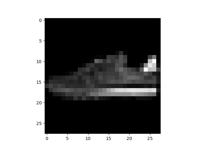
# 读入后,我们可以做一些数据可视化操作,主要是验证我们读入的数据是否正确
image, label = next(iter(train_loader))
print(image.shape, label.shape)
plt.imshow(image[0][0], cmap="gray")
plt.show()
torch.Size([256, 1, 28, 28]) torch.Size([256])
模型构建
由于任务较为简单,这里我们手搭一个 CNN,而不考虑当下各种模型的复杂结构,模型构建完成后,将模型放到 GPU 上用于训练
class Net(nn.Module):
    def __init__(self):
        super(Net, self).__init__()
        self.conv = nn.Sequential(          # 自定义卷积操作,序贯模型
            nn.Conv2d(1, 32, 5),
            nn.ReLU(),
            nn.MaxPool2d(2, stride=2),
            nn.Dropout(0.3),
            nn.Conv2d(32, 64, 5),
            nn.ReLU(),
            nn.MaxPool2d(2, stride=2),
            nn.Dropout(0.3)
        )
        self.fc = nn.Sequential(
            nn.Linear(64*4*4, 512),
            nn.ReLU(),
            nn.Linear(512, 10)              # 10个类别
        )

    def forward(self, x):
        x = self.conv(x)
        x = x.view(-1, 64*4*4)
        x = self.fc(x)
        # x = nn.functional.normalize(x)

model = Net()
model = model.cuda()
# model = nn.DataParallel(model).cuda()     # 多卡训练时的写法
设定损失函数
使用torch.nn模块自带的CrossEntropy损失。PyTorch 会自动把整数型的 label 转为 one-hot 型,用于计算 CE loss。这里需要确保 label 是从
0
0
0 开始的,同时模型不加softmax层(使用logits计算),这也说明了PyTorch训练中各个部分不是独立的,需要通盘考虑
criterion = nn.CrossEntropyLoss()
设定优化器
这里我们使用 Adam 优化器
optimizer = optim.Adam(model.parameters(), lr=0.001)
训练和验证(测试)
训练流程:读取、转换、梯度清零、输入、计算损失、反向传播、参数更新;
验证流程:读取、转换、输入、计算损失、计算指标。
各自封装成函数,方便后续调用。关注两者的主要区别:
- 模型状态设置
- 是否需要初始化优化器
- 是否需要将loss传回到网络
- 是否需要每步更新optimizer
此外,对于测试或验证过程,可以计算分类准确率
def train(epoch):
    model.train()                                        # training mode
    train_loss = 0
    # for i, (datea, label) in enumerate(train_loader):  # batch编号及对应数据
    for data, label in train_loader:
        data, label = data.cuda(), label.cuda()          # 模型在gpu,那么数据也要放在gpu
        optimizer.zero_grad()                            # 梯度清零,防止梯度累加
        output = model(data)                             # 前向传播
        loss = criterion(output, label)                  # 计算损失
        loss.backward()                                  # 沿着计算图进行反向传播
        optimizer.step()                                 # 优化器更新参数
        train_loss += loss.item() * data.size(0)
    train_loss = train_loss / len(train_loader.dataset)  # FMDataset.__len__()
    print('Epoch: {} \tTraining Loss: {:.6f}'.format(epoch, train_loss))

def val(epoch):
    model.eval()                                         # evaluation mode
    val_loss = 0
    gt_labels = []
    pred_labels = []
    with torch.no_grad():                                # 不做梯度计算
        for data, label in test_loader:
            data, label = data.cuda(), label.cuda()
            output = model(data)
            preds = torch.argmax(output, 1)
            gt_labels.append(label.cpu().data.numpy())
            pred_labels.append(preds.cpu().data.numpy())
            loss = criterion(output, label)
            val_loss += loss.item() * data.size(0)
    val_loss = val_loss / len(test_loader.dataset)
    gt_labels, pred_labels = np.concatenate(gt_labels), np.concatenate(pred_labels)
    acc = np.sum(gt_labels == pred_labels) / len(pred_labels)
    print('Epoch: {} \tValidation Loss: {:.6f}, Accuracy: {:.6f}'.format(epoch, val_loss, acc))

for epoch in range(1, epochs+1):
    train(epoch)
    val(epoch)
模型保存
训练完成后,可以使用torch.save保存模型参数或者整个模型,也可以在训练过程中保存模型
save_path = './FashionMNIST.pkl'
torch.save(model, save_path)
我用上述代码保存模型出现了问题,希望大佬能指点一下:
_pickle.PicklingError: Can't pickle <class '__main__.Net'>: attribute lookup Net on __main__ failed
FashionMNIST时装分类代码汇总
# 导入必要的包
import os
import numpy as np
import pandas as pd
import torch
import torch.nn as nn
import torch.optim as optim
from torch.utils.data import Dataset, DataLoader
from torchvision import transforms
import matplotlib.pyplot as plt

# 配置训练环境和超参数
# 配置GPU
os.environ["KMP_DUPLICATE_LIB_OK"] = "TRUE"
os.environ['CUDA_VISIBLE_DEVICES'] = '0'

# 配置其他超参数,如batch_size, num_workers, learning rate, 以及总的epochs
batch_size = 256
num_workers = 0   # 对于Windows用户,这里应设置为0,否则会出现多线程错误
lr = 1e-4
epochs = 20

# 数据读入,自行构建Dataset类,将csv文件中向量形式给出的像素转换成图片形式
# 首先设置数据变换
image_size = 28
data_transform = transforms.Compose([
    transforms.ToPILImage(),         # 这一步取决于后续的数据读取方式,如果使用内置数据集读取方式则不需要
    transforms.Resize(image_size),
    transforms.ToTensor()
])

class FMDataset(Dataset):
    def __init__(self, df, transform=None):
        self.df = df
        self.transform = transform
        self.images = df.iloc[:, 1:].values.astype(np.uint8)    # 读出所有的pixel
        self.labels = df.iloc[:, 0].values                      # 取出标签

    def __len__(self):                                          # 样本数
        return len(self.images)

    def __getitem__(self, idx):                                 # 按idx(index)读取每一张图片
        image = self.images[idx].reshape(28, 28, 1)             # 向量→图片,width*height*channel=28*28*1
        label = int(self.labels[idx])
        if self.transform is not None:
            image = self.transform(image)
        else:
            image = torch.tensor(image / 255., dtype=torch.float)
        label = torch.tensor(label, dtype=torch.long)
        return image, label


train_df = pd.read_csv("E:\\Code\\pythonProject\\pytorchBase\\FashionMNIST\\fashion-mnist_train.csv")
test_df = pd.read_csv("E:\\Code\\pythonProject\\pytorchBase\\FashionMNIST\\fashion-mnist_test.csv")
train_data = FMDataset(train_df, data_transform)
test_data = FMDataset(test_df, data_transform)

# 在构建训练和测试数据集完成后,需要定义DataLoader类,以便在训练和测试时加载数据
train_loader = DataLoader(train_data, batch_size=batch_size, shuffle=True, num_workers=num_workers, drop_last=True)
test_loader = DataLoader(test_data, batch_size=batch_size, shuffle=False, num_workers=num_workers)

# # 读入后,我们可以做一些数据可视化操作,主要是验证我们读入的数据是否正确
# image, label = next(iter(train_loader))   # 从dataloader中取到一个数据
# print(image.shape, label.shape)
# plt.imshow(image[0][0], cmap="gray")
# plt.show()

# 模型构建
class Net(nn.Module):
    def __init__(self):
        super(Net, self).__init__()         # 注意是 __init__(),不要错打成__int__()
        self.conv = nn.Sequential(          # 自定义卷积操作,序贯模型
            nn.Conv2d(1, 32, 5),
            nn.ReLU(),
            nn.MaxPool2d(2, stride=2),
            nn.Dropout(0.3),
            nn.Conv2d(32, 64, 5),
            nn.ReLU(),
            nn.MaxPool2d(2, stride=2),
            nn.Dropout(0.3)
        )
        self.fc = nn.Sequential(
            nn.Linear(64*4*4, 512),
            nn.ReLU(),
            nn.Linear(512, 10)              # 10个类别
        )

    def forward(self, x):
        x = self.conv(x)
        x = x.view(-1, 64*4*4)
        x = self.fc(x)
        # x = nn.functional.normalize(x)
        return x                            # 别忘了

model = Net()
model = model.cuda()
# model = nn.DataParallel(model).cuda()     # 多卡训练时的写法

# 设定损失函数
criterion = nn.CrossEntropyLoss()

# 设定优化器
optimizer = optim.Adam(model.parameters(), lr=0.001)

# 训练和测试(验证)
def train(epoch):
    model.train()                                        # training mode
    train_loss = 0
    # for i, (datea, label) in enumerate(train_loader):  # batch 编号及对应数据
    for data, label in train_loader:
        data, label = data.cuda(), label.cuda()          # 模型在gpu,那么数据也要放在gpu
        optimizer.zero_grad()                            # 梯度清零,防止梯度累加
        output = model(data)                             # 前向传播
        loss = criterion(output, label)                  # 计算损失
        loss.backward()                                  # 沿着计算图进行反向传播
        optimizer.step()                                 # 优化器更新参数
        train_loss += loss.item() * data.size(0)
    train_loss = train_loss / len(train_loader.dataset)  # FMDataset.__len__()
    print('Epoch: {} \tTraining Loss: {:.6f}'.format(epoch, train_loss))

def val(epoch):
    model.eval()                                         # evaluation mode
    val_loss = 0
    gt_labels = []
    pred_labels = []
    with torch.no_grad():                                # 不做梯度计算
        for data, label in test_loader:
            data, label = data.cuda(), label.cuda()
            output = model(data)
            preds = torch.argmax(output, 1)
            gt_labels.append(label.cpu().data.numpy())
            pred_labels.append(preds.cpu().data.numpy())
            loss = criterion(output, label)
            val_loss += loss.item() * data.size(0)
    val_loss = val_loss / len(test_loader.dataset)
    gt_labels, pred_labels = np.concatenate(gt_labels), np.concatenate(pred_labels)
    acc = np.sum(gt_labels == pred_labels) / len(pred_labels)
    print('Epoch: {} \tValidation Loss: {:.6f}, Accuracy: {:.6f}'.format(epoch, val_loss, acc))


if __name__ == '__main__':
    for epoch in range(1, epochs+1):
        train(epoch)
        val(epoch)

    # # jupyternotebook 查看Gpu的写法
    # gpu_info = !nvidia-smi -i 0
    # gpu_info = '\n'.join(gpu_info)
    # print(gpu_info)

    # 模型保存
    save_path = './FashionMNIST.pkl'
    torch.save(model, save_path)


 5万+
5万+

 被折叠的 条评论
为什么被折叠?
被折叠的 条评论
为什么被折叠?
 到【灌水乐园】发言


