【Python】Section 7: Bootstrap, 置信区间和假设检验 from HarvardX

Yqalu

已于 2024-05-01 17:17:52 修改

阅读量1k

点赞数 28

分类专栏： HarvardX CS109x 文章标签： python 数据分析机器学习

于 2024-05-01 17:15:05 首次发布

本文链接：https://blog.csdn.net/Yqalu/article/details/138375414

版权

HarvardX CS109x 专栏收录该内容

8 篇文章 0 订阅

订阅专栏

1. Inference in Linear Regression

After fitting a linear regression model we often look at the coefficients to infer relationships between the predictors and the response variable. But we should always ask, "how reliable are our model interpretations?"

Suppose our model for advertising:

$y=1.01x+120$

Here x are in $1000s and y are in thousand unit sales and every unit sells for $1.

Our interpretation might then be as follows: for every dollar invested in advertising, we get an additional 1.01 back in sales. That is, 1% profit.

1.1 Confidence intervals for the predictors estimates

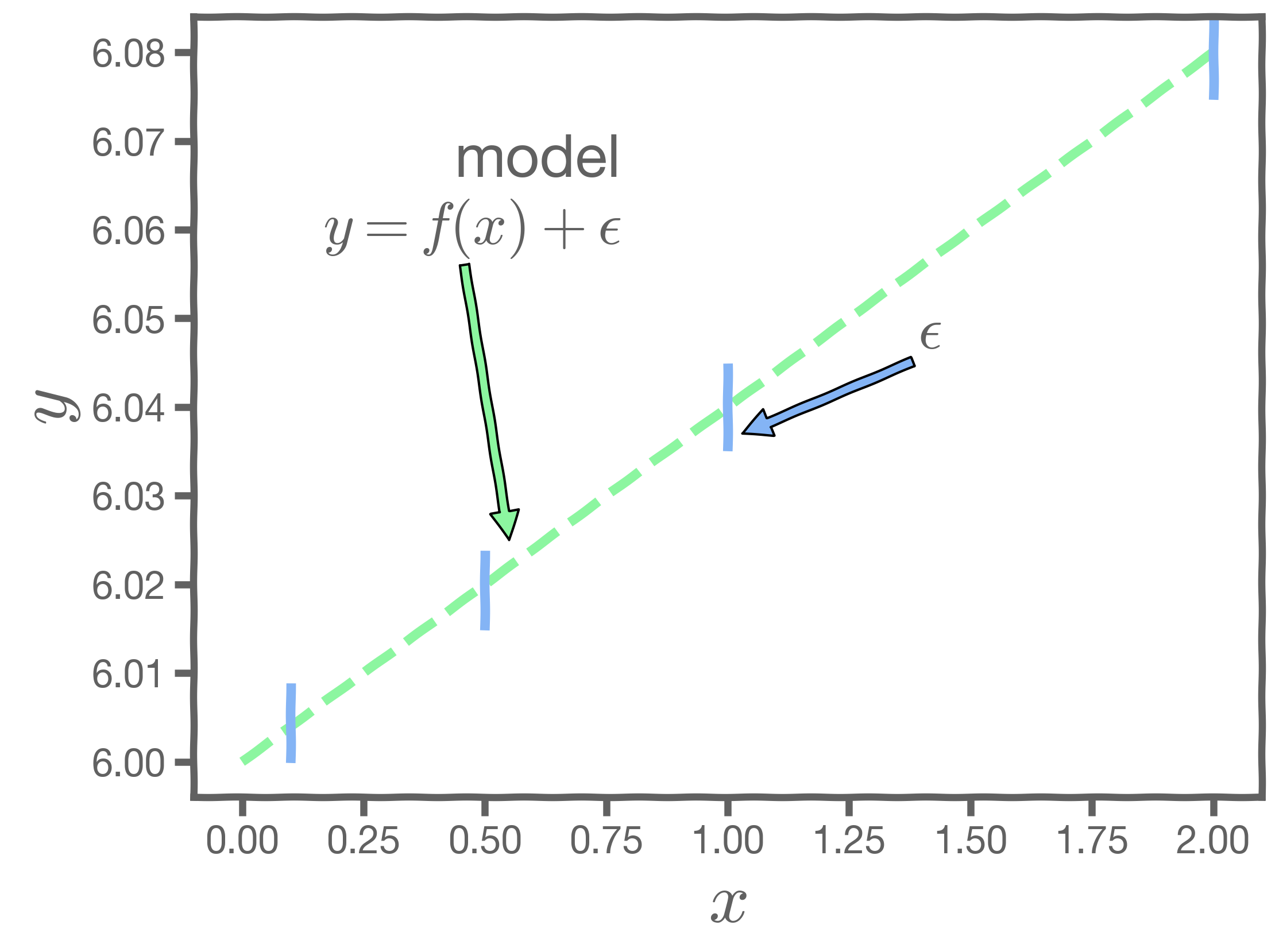
Our observation, represented as $y=f(x)+\epsilon$ , is interpreted either as the noise introduced by random variations in natural systems, or imprecisions of the measuring instruments, or environmental irregularities.

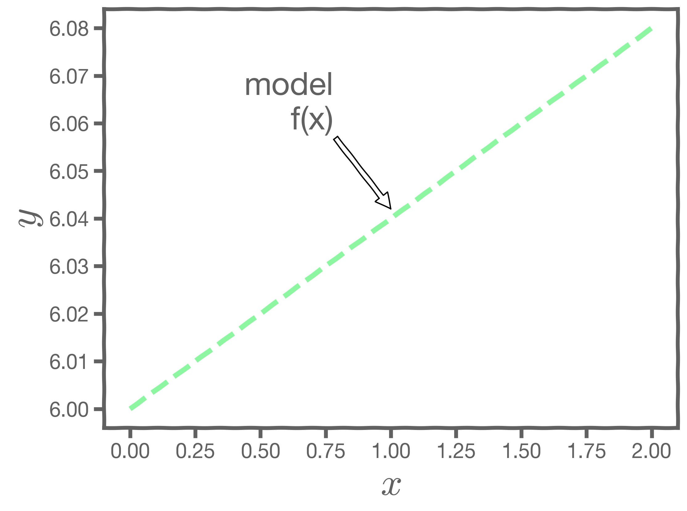
If we knew the exact form of $f(x)$ ,for example, $f(x)=\beta_0+\beta_1(x)$ , and there was no noise in the data, then the estimation of would have been exact.

A straight line that goes perfectly through 7 data points.

In such a case, is a 1% profit worth it? That's a business decision, and not one that linear regression can answer.

However, two things should make us mistrust of the values of $\widehat{\beta}s$ :

observational error is always there - this is called aleatoric error or irreducible error
the exact form of $f(x)$ is unknown - this is called misspecification error and is part of the epistemic error

Both errors are combined into a catch-it-all term, . Because of this, every time we measure the response $y$ for a fixed value of $x$ , we will obtain a different observation and hence a different estimate of $\widehat{\beta}s$ .

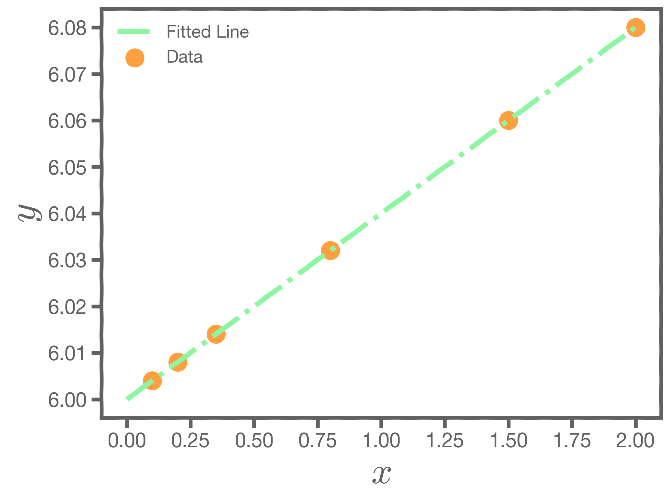
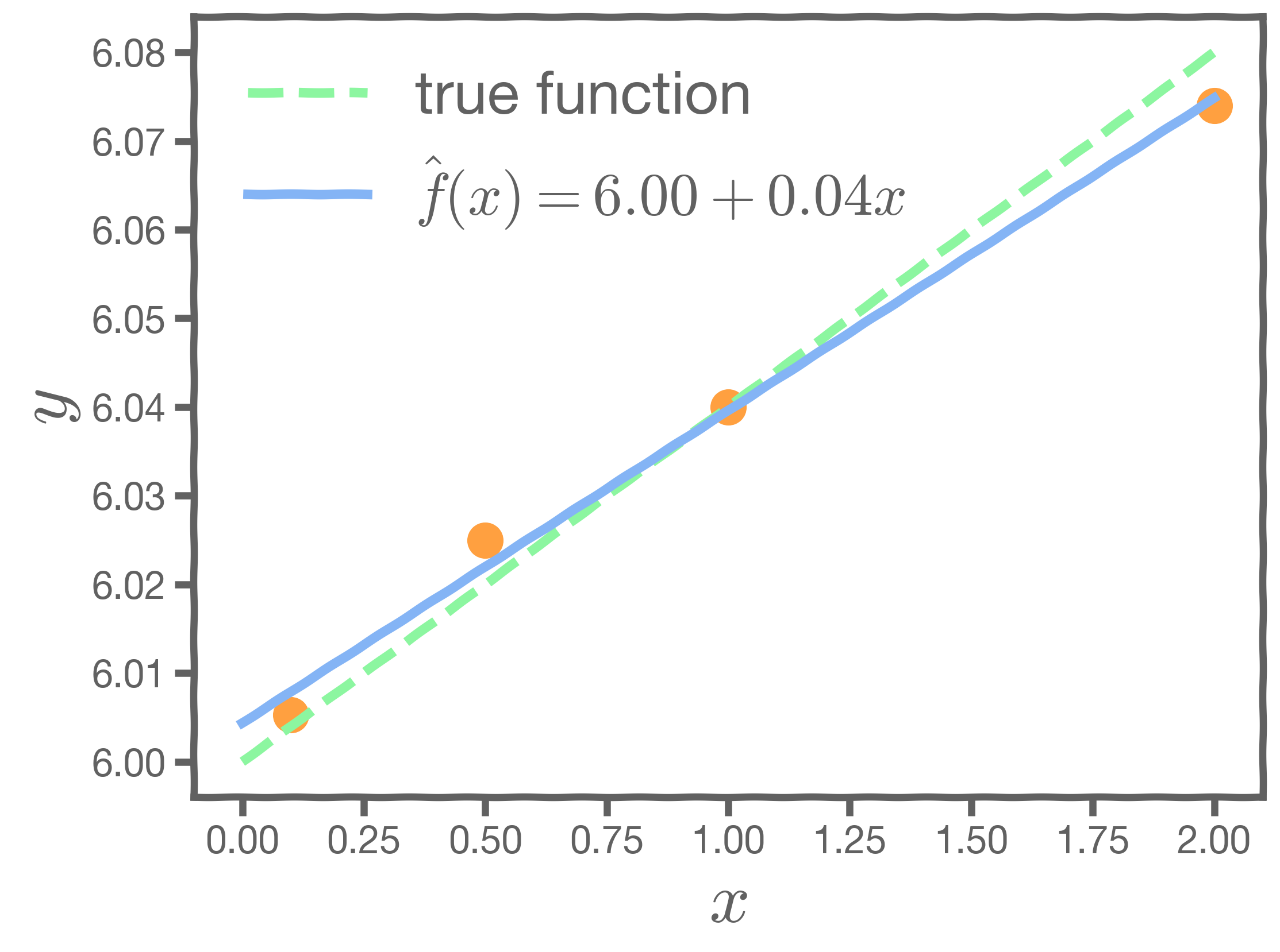
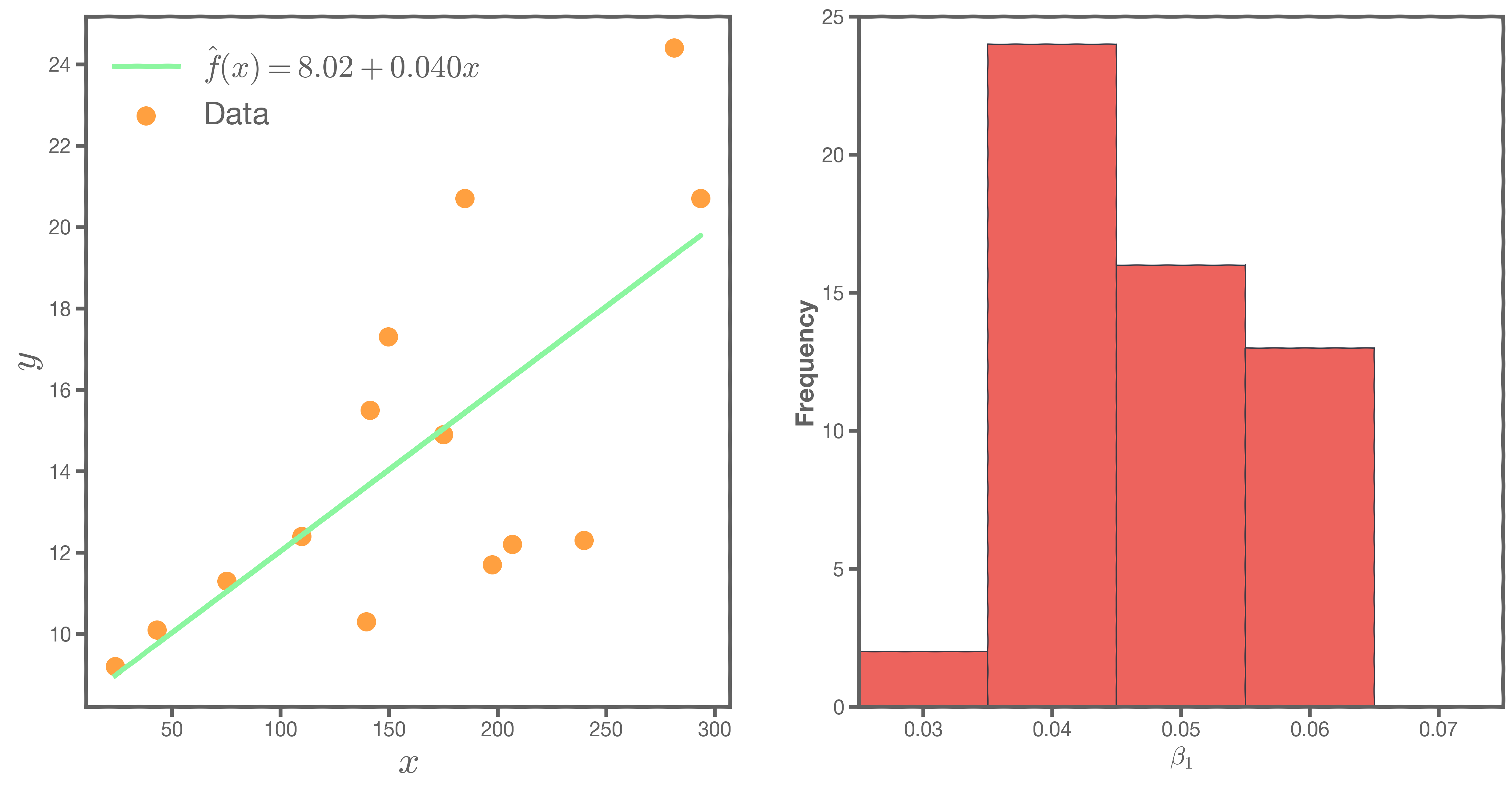
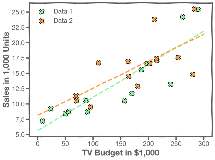
Let us consider an example. Start with a model $f(X)$ , the correct relationship between input and outcome.

A linear model - a straight line on a graph of y vs x.

For some values of $x$ , $Y=f(X)$

The same line with a set of predicted values indicated. The predicted values are on the line.

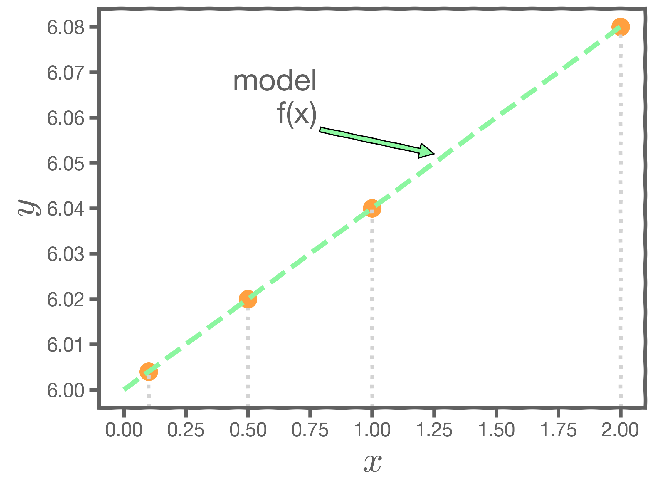
Every time we measure the response $Y$ for a fixed $X$ we obtain a different observation.

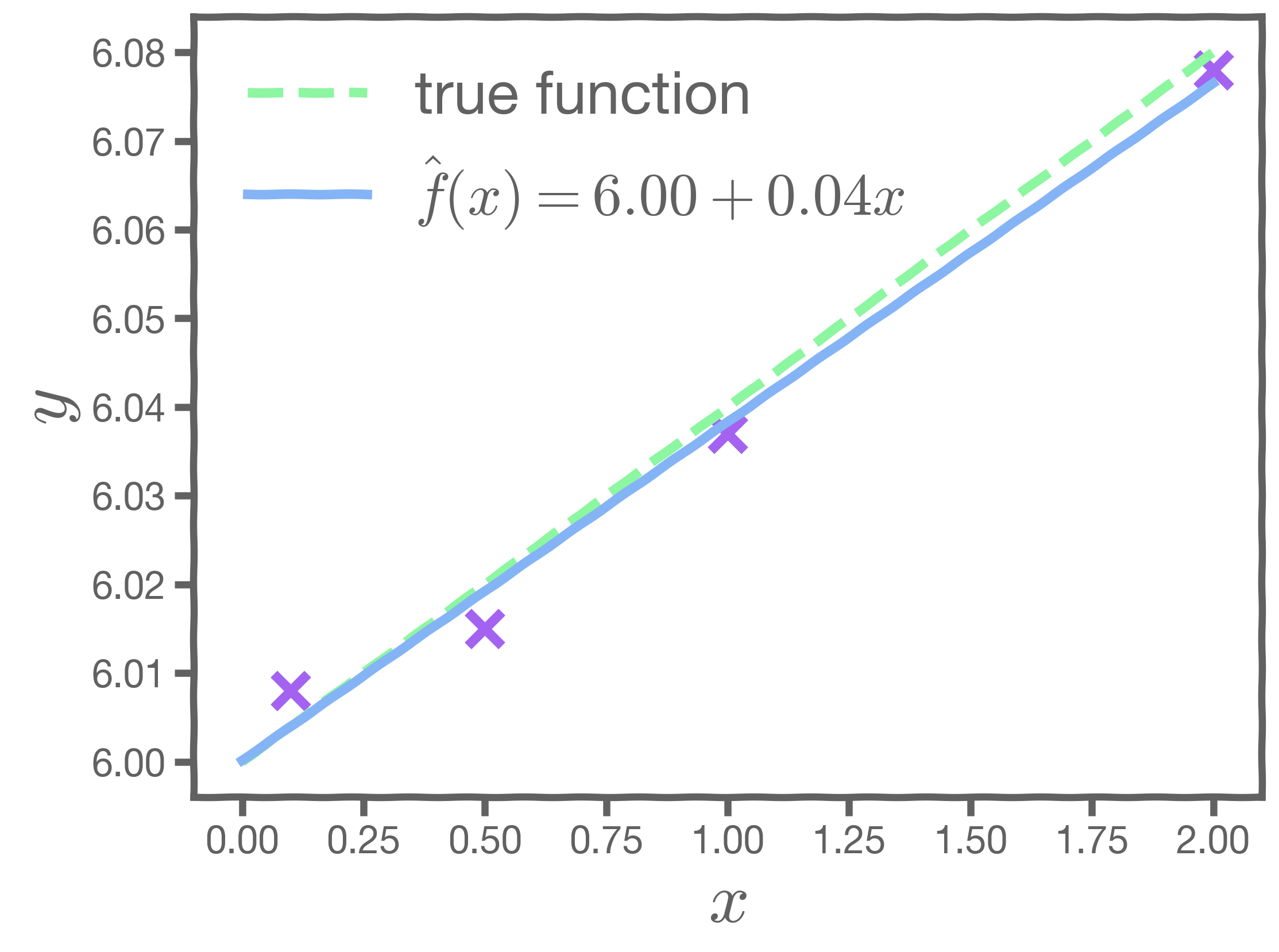
The same predicted values, but with error bars indicated to show the range of likely values.

One set of observations, "one realization" yields one set of $Y$ . This is represented as orange circles in the plot. Similarly, the squares and crosses each represent a set of $Y$ realized.

The same value ranges. Multiple sets of observations, or realizations, of the data are shown.

For each of these realizations, we fit a model and estimate $\widehat{\beta}_0$ and $\widehat{\beta}_1$ . Thus, it results in one set of model parameters, $\widehat{\beta}_0$ and $\widehat{\beta}_1$ , for each realization.

A best-fit line for one of the realizations of the data.

A best-fit line for a different realization of the data.

So, if we have one set of measurements of $X,Y$ , our estimates of $\widehat{\beta}_0$ and $\widehat{\beta}_1$ are just for this particular realization. Given this, how do we know the truth? How do we deal with this conundrum?

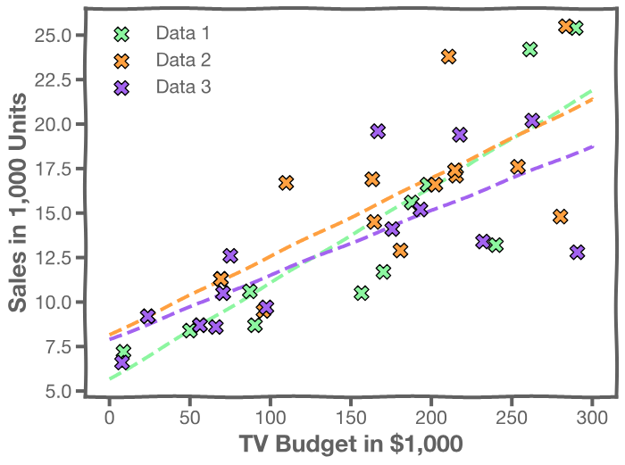
To resolve this, imagine that we have a multitude of parallel universes, and we repeat this experiment on each of the other universes.

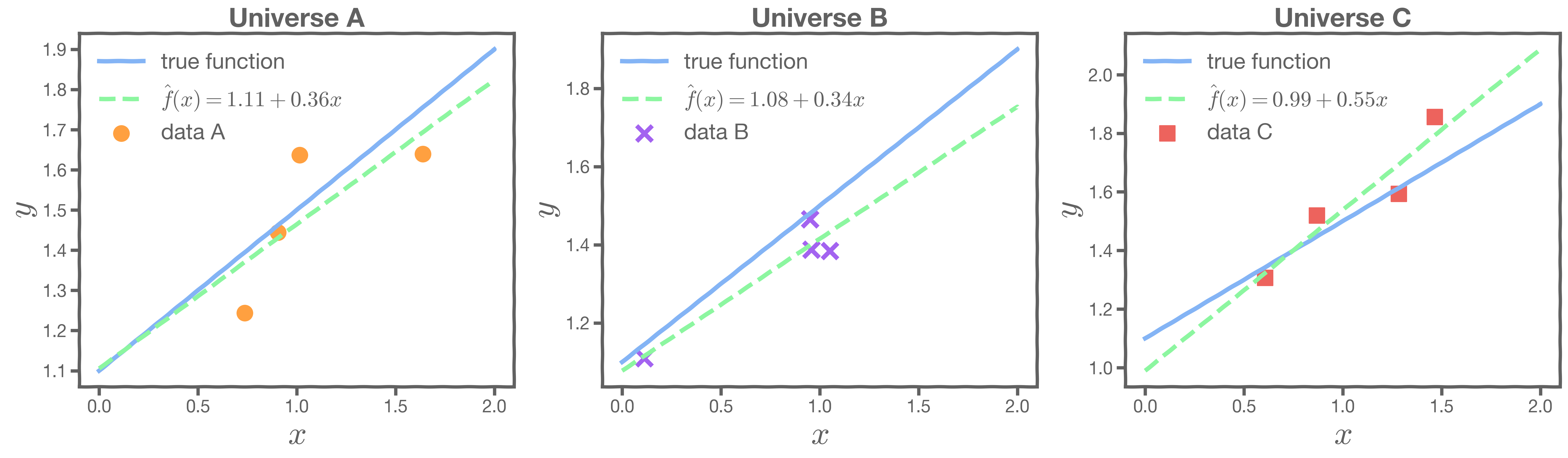
Multiple best-fit graphs, each fitting a different universe's data.

In our magical realism, we can now sample $X,Y$ multiple times. One universe means one sample, which means one set of estimates for $\widehat{\beta}_0$ and $\widehat{\beta}_1$ . The graphs on the left below show the best-fit lines for each of the universes, and the right-hand graph shows the distribution of the estimates of $\widehat{\beta}_0$ and $\widehat{\beta}_1$ .

A single best-fit line, with a single block added to the histogram.

Another sample, another estimate of $\widehat{\beta}_0$ and $\widehat{\beta}_1$

A different best-fit to a different sample of data, with a second block added to the histogram.

This is repeated until we have sufficient samples of $\widehat{\beta}_0$ and $\widehat{\beta}_1$ to understand their distribution.

The Nth best-fit line. The histogram has many blocks now, showing the distribution of the data.

2. Bootstrap and Confidence Intervals

2.1 Producing Alternative Data Sets

In the absence of active imagination, magic, parallel universes, and the like, we need an alternative way of producing fake data sets that resemble parallel universes.

Bootstrapping is the practice of sampling observed data to estimate statistical properties.

Bootstrap Example

A bucket with five billiard balls.

We first randomly pick a ball and replicate it. We then move the replicated ball to another bucket.

An animation: one ball is copied, and the copy moves from the original bucket to a new one.

This is called sampling with replacement.
We then randomly pick another ball and replicate it again. As before, we move the replicated ball to the other bucket.

Another ball is copied and moved to the new bucket. The same balls are still in the original bucket.

We repeat this process. We continue until the 'other' bucket has the same number of balls as the original.

Both buckets now contain five balls.

We repeat the same process and acquire many sets of bootstrapped observations.

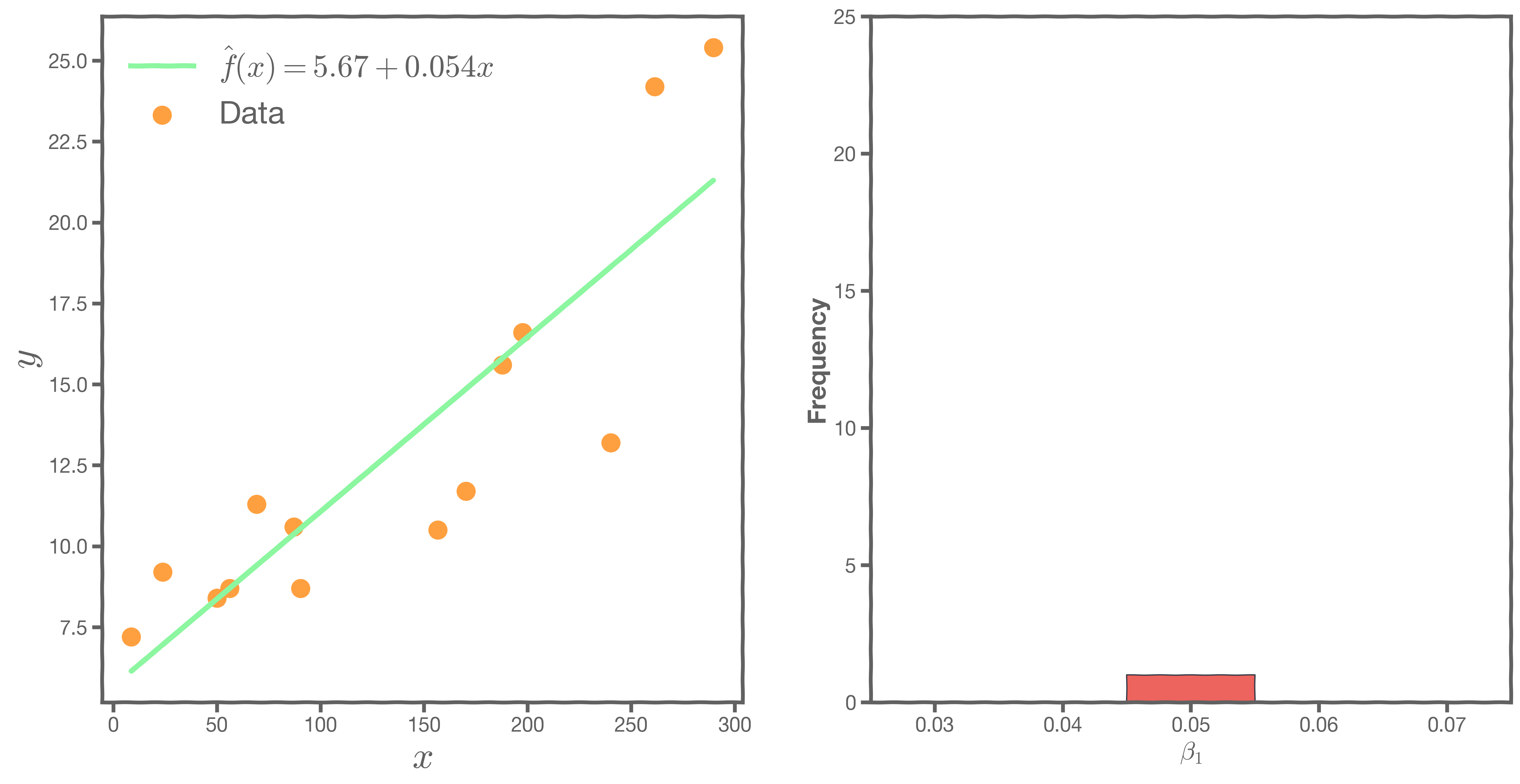
The process repeats for multiple buckets.

2.2 Bootstrapping for Estimating Sampling Error

Bootstrapping is the practice of estimating the properties of an estimator by measuring those properties by, for example, sampling from the observed data. For example, we can compute $\widehat{\beta}_0$ and $\widehat{\beta}_1$ multiple times by randomly sampling our data set. We then use the variance of our multiple estimates to approximate the true variance of $\widehat{\beta}_0$ and $\widehat{\beta}_1$ .

The process is repeated many times. The collection of bootstrap samples is used to provide calculate the standard deviation for the model's beta values.

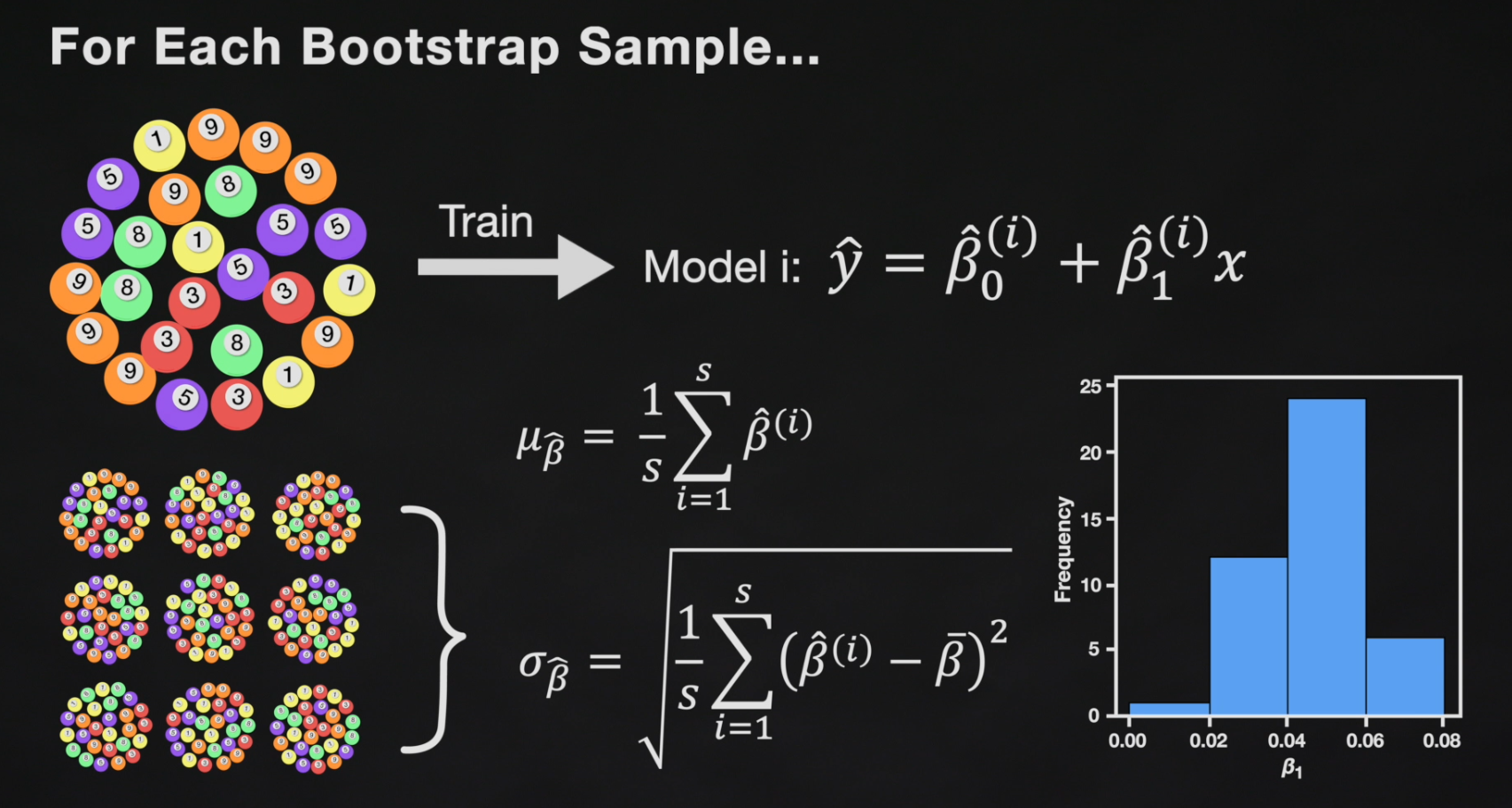
We can now estimate the mean and standard deviation of the estimates and .

$\widehat{y}=\widehat{\beta}_0^{(i)}+\widehat{\beta}_1^{(i)}x$

$\mu _{\widehat{\beta}}=\frac{1}{s}\sum_{i=1}^{s}\widehat{\beta}^{(i)}$

$\sigma _{\widehat{\beta}}=\sqrt{\frac{1}{s}\sum_{i=1}^{s}(\widehat{\beta}^{(i)}-\overline{\beta})}$

The standard errors give us a sense of our uncertainty over our estimates. Typically, we express this uncertainty as a 95% confidence interval, which is the range of values such that the true value of $\beta_1$ is contained in this interval with 95% percent probability.

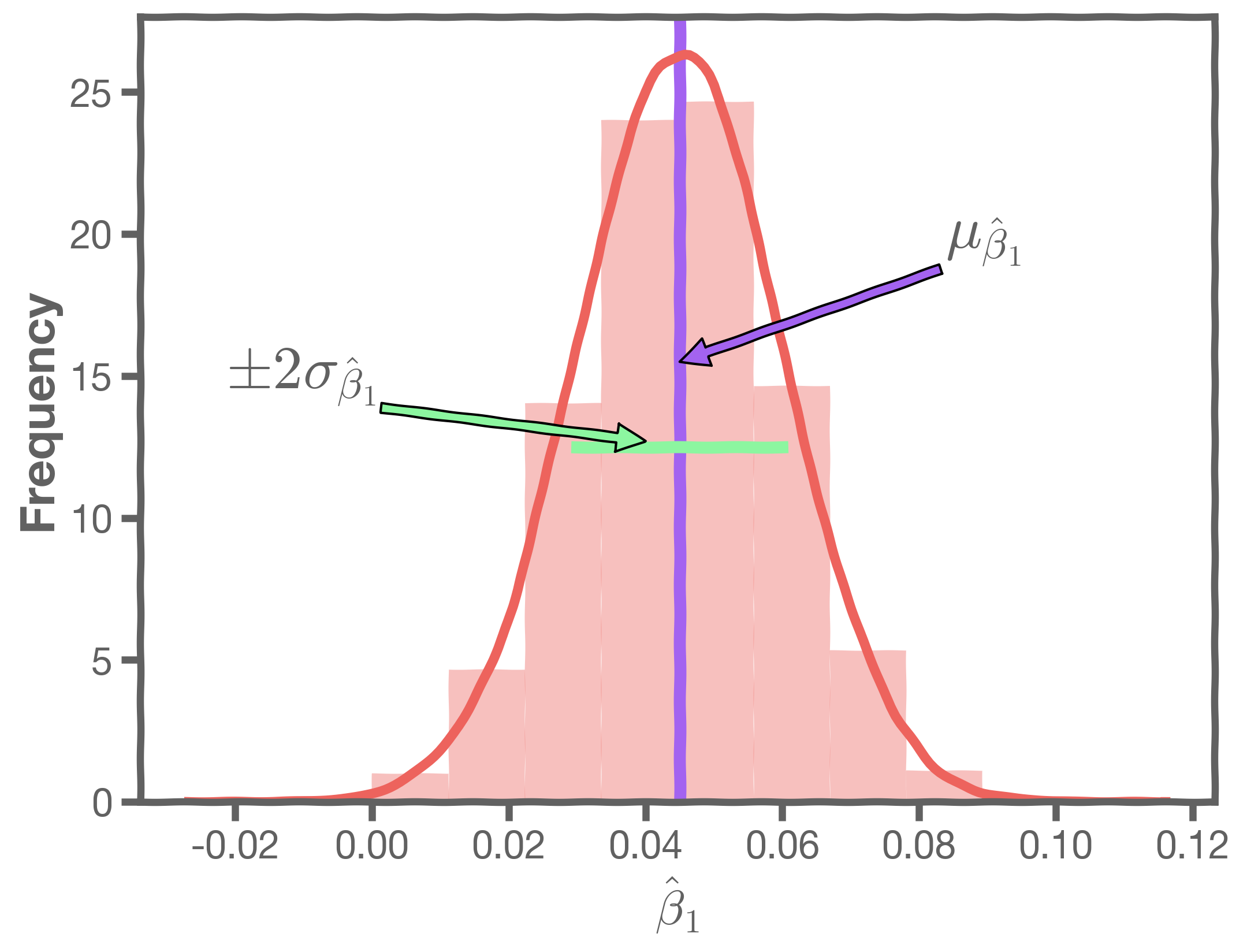
A typical gaussian distribution with values of mu beta and sigma beta shown.

If we assume normality, then:

$CI_{\widehat{\beta}}\left ( 95\% \right )=(\widehat{\beta}-2\sigma _{\widehat{\beta}},\widehat{\beta}+2\sigma _{\widehat{\beta}})$

3. Evaluating Predictor Significance

3.1 Feature importance

Now that we know how to generate these distributions we are ready to answer two important questions:

Which predictors are most important?
which of them really affects the outcome?

The three charts below show three different histograms for beta, for newspaper, TV, and radio advertising. Each one has a different mean and standard deviation. How can we tell which of these three predictors is the most important?

To incorporate the uncertainty of the coefficients, we need to determine whether the estimates of 's are sufficiently far from zero.

To do so, we define a new metric, which we call $\widehat{t}$ -test statistic:

The $\widehat{t}$ -test

The -test statistic measures the distance from zero in units of standard deviation.

$\widehat{t}-test=\frac{\mu _{\widehat{\beta}_1}}{\sigma _{\widehat{\beta}_1}}$

$\widehat{t}$ -test is a scaled version of the usual t-test,

$\widehat{t}-test=\frac{\mu _{\widehat{\beta}_1}}{\sigma _{\widehat{\beta}_1}/\sqrt{n}}=\sqrt{n}-test$

where $n$ is the number of bootstraps.

3.2 Feature Importance

Consider the following example using the Boston Housing data. This dataset contains information collected by the U.S Census Service concerning housing in the area of Boston. The coefficients below are from a model that predicts prices given house size, age, crime, pupil-teacher ratio, etc.

This plot gives the feature importance based on the absolute value of the coefficients.

A bar graph of the absolute values of various predictors.

The following plot gives the feature importance based not on the absolute value of the coefficients over multiple bootstraps and includes the uncertainty of the coefficients.

The same graph, with error bars shown for the uncertainty.

Finally, we have the feature importance based on the t-test. Notice that the rank of the importance has changed.

A similar-looking graph, but with the features in a different order - their relative importance has changed.

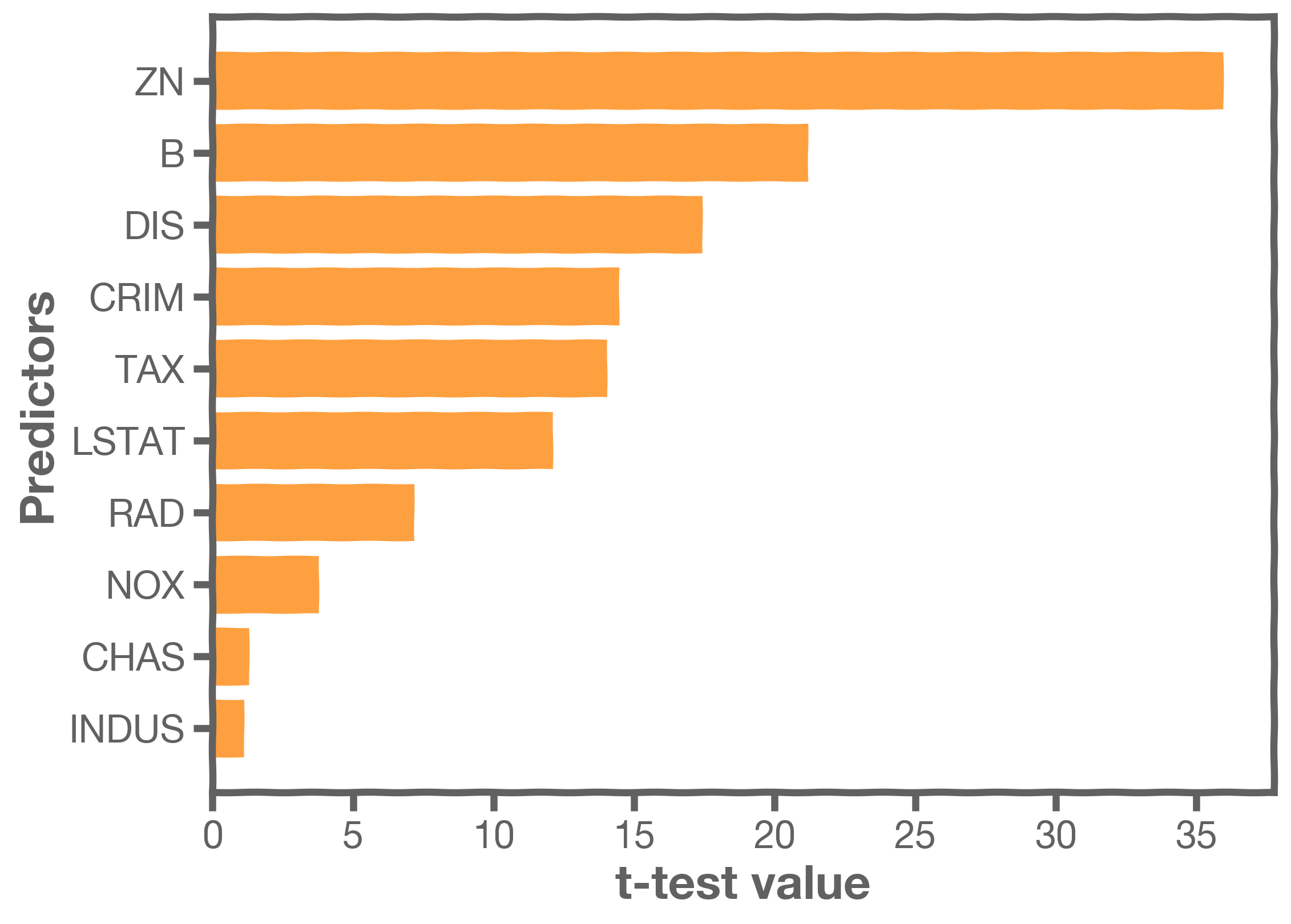
Just because a predictor is ranked as the most important, it does not necessarily mean that the outcome depends on that predictor. How do we assess if there is a true relationship between outcome and predictors?

As with R-squared, we should compare its significance $\widehat{t}$ -test to the equivalent measure from a dataset where we know that there is no relationship between predictors and outcome.

We are sure that there will be no such relationship in data that are randomly generated. Therefore, we want to compare the $\widehat{t}$ -test of the predictors from our model with -test values calculated using random data using the following steps:

For random datasets fit models
Generate distributions for all predictors and calculate the means and standard errors
Calculate the t-tests
Repeat and create a Probability Density Function (PDF) for all the t-tests

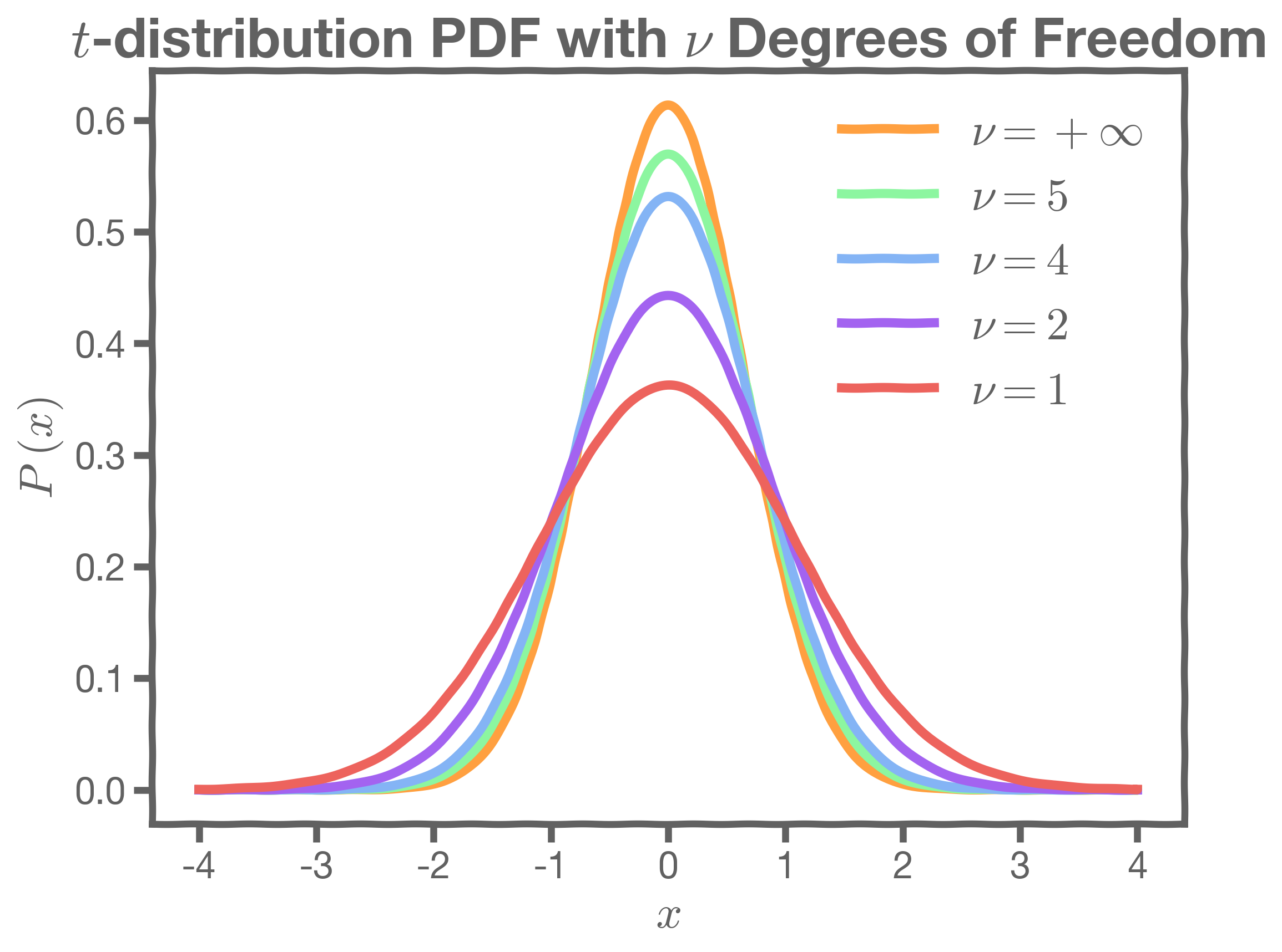
It turns out we do not have to of this, because this is a known distribution called student-t distribution.

In this student-t distribution plot, represents the degrees of freedom (number of data points minus number of predictors):

A graph with several bell-like curves. The higher the value of nu, the narrower the curve becomes.

3.3 P-value

To compare the t-test values of the predictors form our model, , we estimate the probability of observing . This is called the probability of the p-value, defined as:

P-value

$p-value=P(\left | t^R \right | \geq\left | t^* \right |)$

A small p-value indicates that it is unlikely to observe such a substantial association between the predictor and the response due to chance.
It is common practice to use p-value < 0.05 as the threshold for significance.
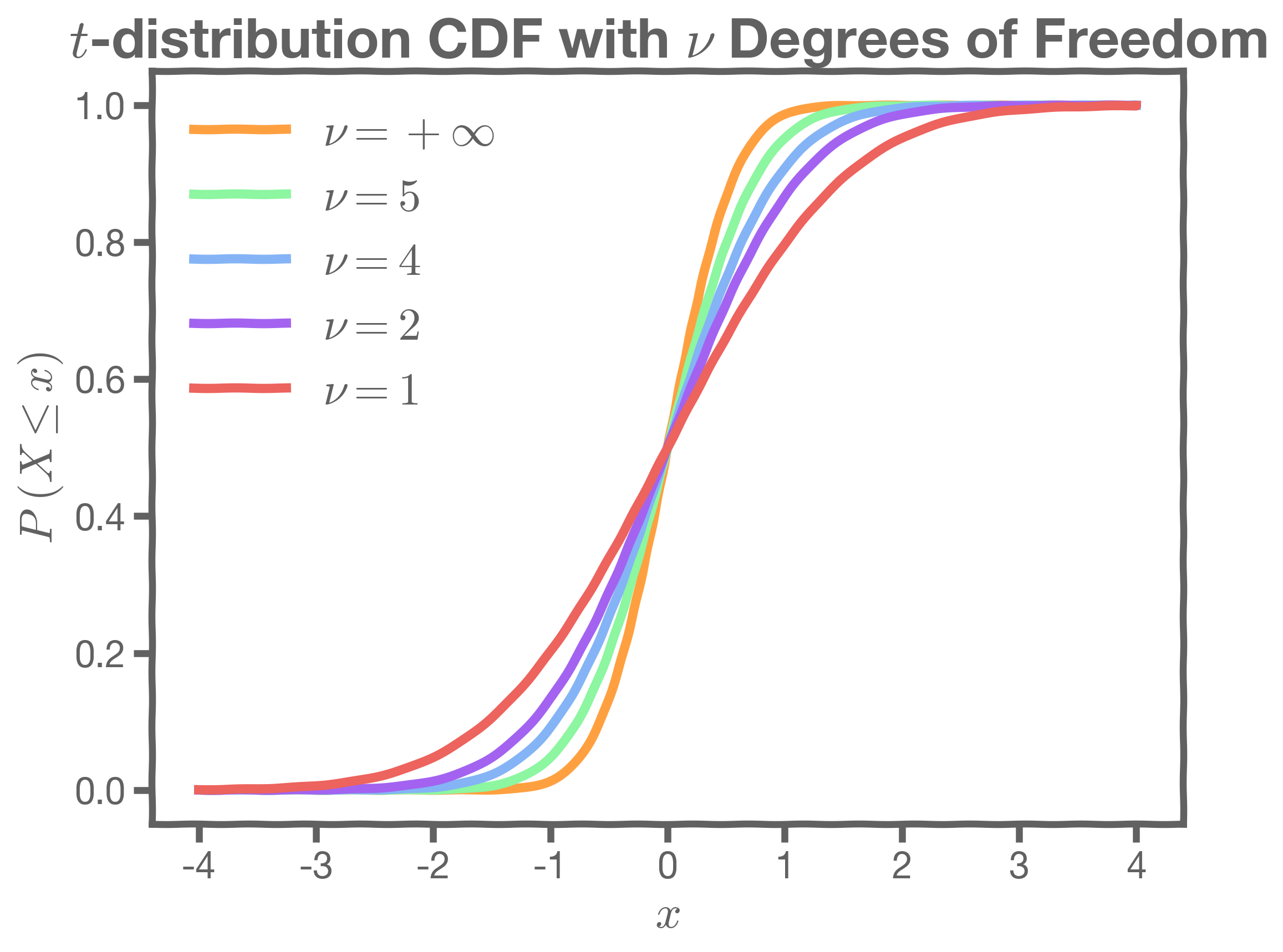
NOTE: To calculate the p-value we use the Cumulative Distribution Function (CDF) of the student-t.

stats model a Python library has a build-in function stats.t.cdf() which can be used to calculate this.

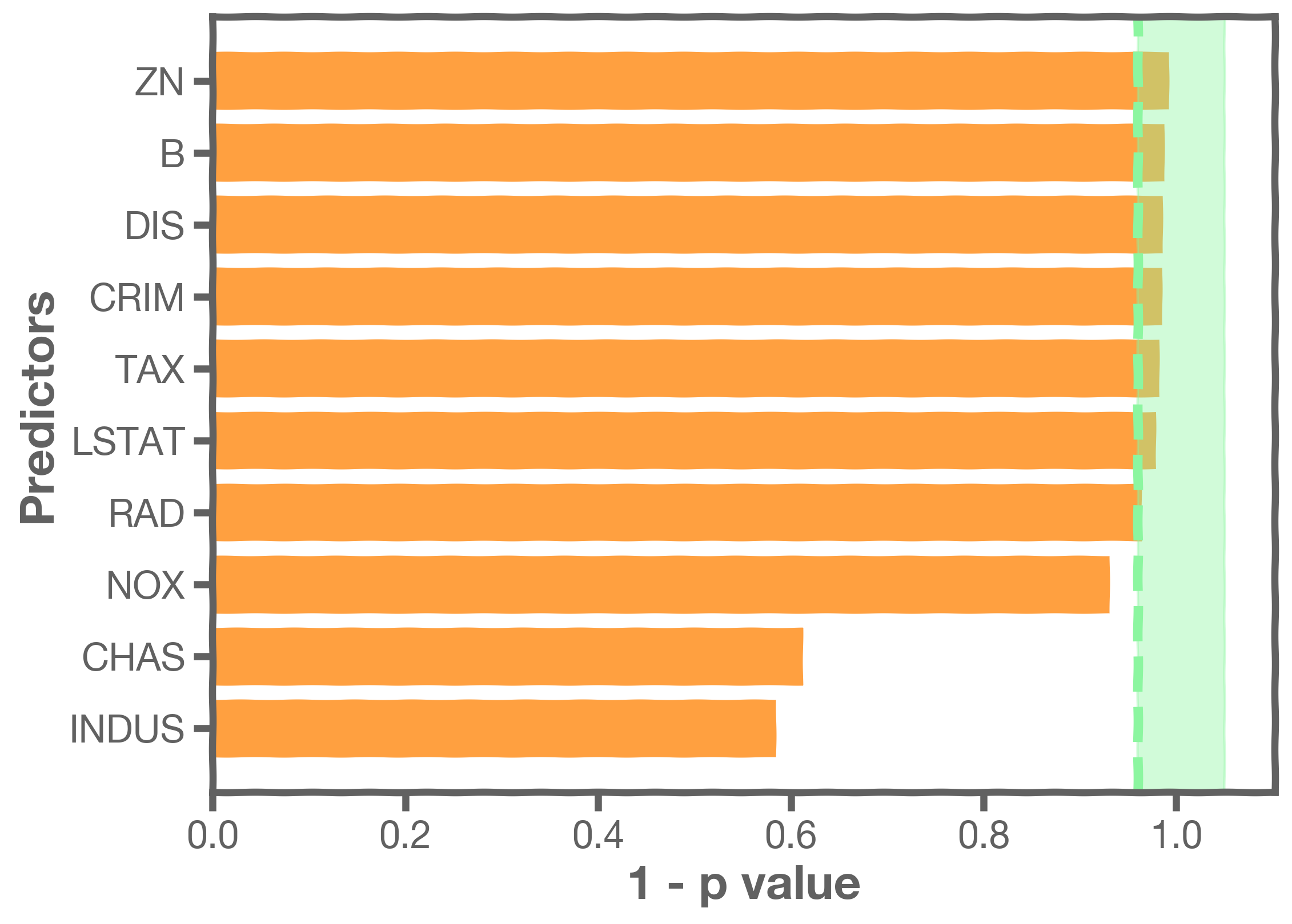
A graph with several logistic curves. The higher the value of nu, the steeper the curve becomes.

As a continuation of the Boston Housing data example used above, we now have the feature importance plotted using the p-value.

Another graph with the features in a different order - their relative importance has changed again. A region is shaded in to show the predictors with the lowest p-vales.

3.4 Hypothesis Testing

Hypothesis testing is a formal process through which we evaluate the validity of a statistical hypothesis by considering evidence for or against the hypothesis gathered by random sampling of the data.

The involves the following steps:

State the hypothesis, typically a null hypothesis, $H_0$ and an alternative hypothesis, $H_1$ , that is the negation of the former.
Choose a type of analysis, i.e. how to use sample data to evaluate the null hypothesis. Typically this involves choosing a single test statistic.
Sample data and compute the test statistic.

Use the value of the test statistic to either reject or not reject the null hypothesis.

This is an example of the Hypothesis testing process:

1. State Hypothesis
  - Null hypothesis: $H_0$ : There is no relation between $X$ and $Y$
  - Alternative hypothesis: $H_0$ : There is some relation between $X$ and $Y$
2. Choose Test Statistic: the t-test
3. Sample: Using bootstrapping we can estimate $\widehat{\beta}_1$ s, $\mu _{\widehat{\beta}_1}$ , $\sigma _{\widehat{\beta}_1}$ and the t-test
4. Reject or accept the hypothesis
  - We compute the p-value, the probability of observing any value equal to or larger from random data.
    - If p-value < (p-value - threshold), reject the null hypothesis
    - Else, accept the null hypothesis

4. Prediction Intervals

4.1 How well do we know $\widehat{f}$ ?

Our confidence in $f$ is directly related to the confidence in , which we can use to determine the model $f(x)=X\beta$

Here we show one models' predictions given the fitted coefficients.

Here is another one.

There is one such regression line for every bootstrapped sample.

The following plot shows all regression lines for 1,000 such bootstrapped samples.

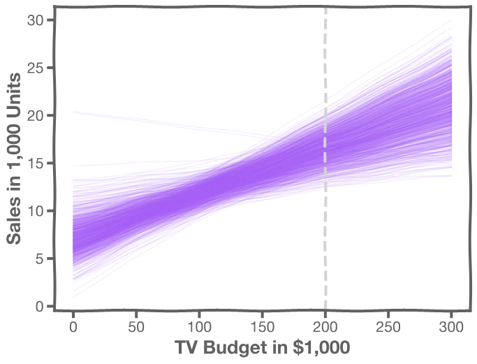
For a given $x$ , we examine the distribution of $\widehat{f}$ and determine the mean and standard deviation.

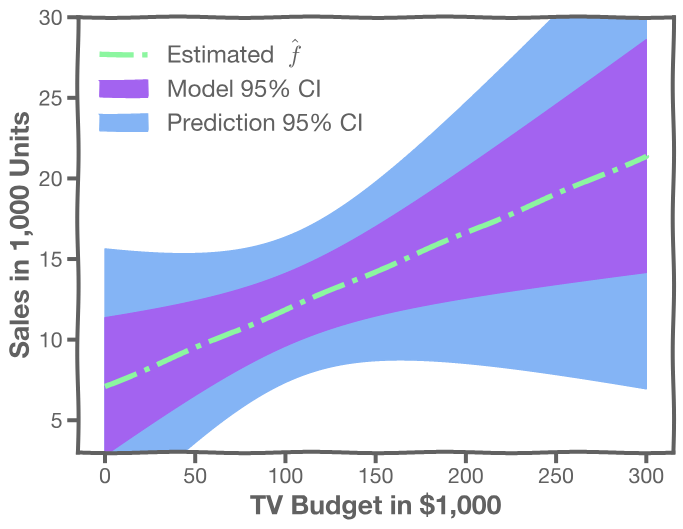
For every $x$ , we calculate the mean and standard deviation of the models, (shown with dotted line) and the 95% CI of those models (shaded area)

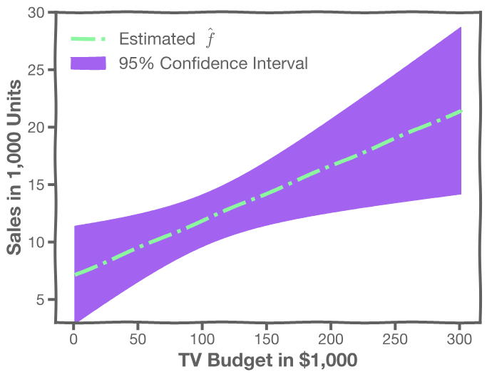
4.2 Confidence in predicting $\widehat{y}$

Even if we know - the response value cannot be perfectly predicted because of the random error in the model (irreducible error).

To find out how much $Y$ will vary from $\widehat{Y}$ , we use prediction intervals.

The prediction interval is obtained using the following method:

For a given , we have a distribution of models $f(x)$
For each of these $f(x)$ , the prediction for $y\approx N(f(x),\sigma _\epsilon )$
The prediction confidence intervals are then the 95% region as depicted in the plot

Yqalu

关注

28
点赞
踩
11

收藏

觉得还不错? 一键收藏
1
评论
【Python】Section 7: Bootstrap, 置信区间和假设检验 from HarvardX

HarvardX CS109x "Introduction to Data Science with Python"\Section 7: Bootstrap, Confidence Intervals, and Hypothesis Testing
复制链接

扫一扫