一篇文章真正讲懂模型评估指标(准确率，召回率，精确率，roc曲线，AUC值）

背景：

最近在做一些数据分析的比赛的时候遇到了一些头疼的问题，就是我们如何评估一个模型的好坏呢？

准确率，召回率，精确率，roc曲线，roc值等等，但是模型评估的时候用哪个指标呢，在此出一篇文章仔细说一说吧，希望大家看完能有收获！

模型评估

我们先从会混淆矩阵说起。

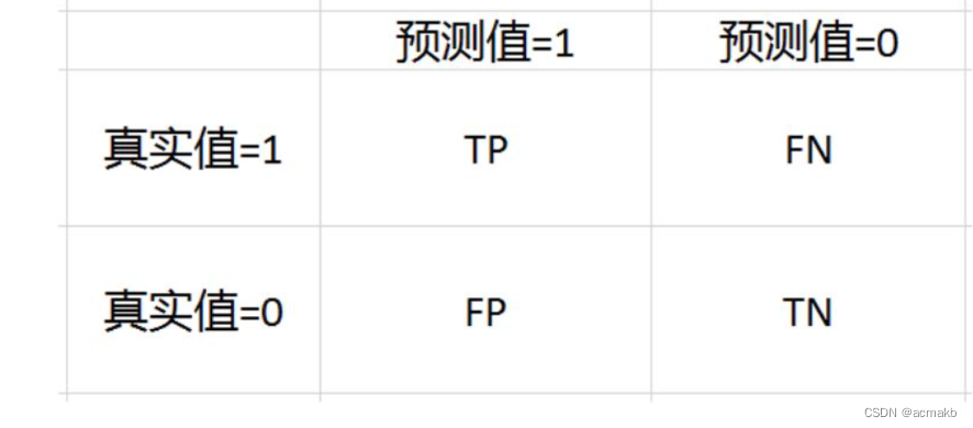
这个是一个二分类混淆矩阵，也是我们真实值和预测值的对应关系.

True False 代表真实值和预测值是否相同。

• True Positive（TP）：真实为正，预测为正 ----------------真的真
• False Negative（FN）：真实为正，预测为反 -----------假的假 -------也就是说不是假的 也就是真的
• False Positive（FP）：真实为假，预测为正 --------------假的真 -----也就是说应该是不是真的
• True Negative（TN）：真实为假，预测为假 ------------------ 真的假

我觉得这样子的解释大家应该比较容易理解吧.

接下来是基于这个四个的指标：

精确率：

即对的概率：真的假和真的真 占全体的比例。

这个指标表示模型预测正确的概率，精度越高，模型越优秀。
$$Accuracy=(TP+TN)/(TP+FN+FP+TN)$$

正确率：

即 在预测为真的情况下，预测正确的概率。
$$Precision=TP/(TP+FP)$$

召回率：

即 在真实为真的情况下，能预测成功的概率
$$Recall=TP/(TP+FN)$$

召回率和正确率的区别：

注意区分正确率和召回率，分子相同 ，但是分母一个是相对于 真实值为真来说的， 一个是相对于预测值为真来说的

特异性：

即 在真实为假的条件下 预测为假 。

$$FPR=TN/(TN+FP)$$

负正类率：

即 在真实为假的条件下 预测为真 。

其实就是预测错了。
$$FPR=FP/(TN+FP)$$

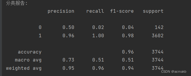
分类报告：

这个报告会包括很多值，可以展示出 precision recall f1-score support 等等，如下.

ROC曲线：

ROC曲线解释：

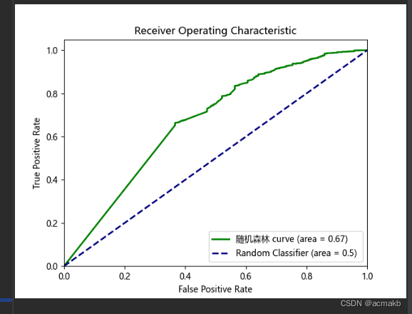
​ ROC曲线是评估二分类模型性能的常用工具。在ROC曲线中，横轴表示模型的假阳性率（False Positive Rate，FPR），纵轴表示模型的真阳性率（True Positive Rate，TPR），也可以称为灵敏度（Sensitivity）或召回率（Recall）。

​ ROC曲线以不同的分类阈值为基础，绘制了模型在不同阈值下的TPR和FPR。曲线上的每个点代表了模型在特定阈值下的性能，而曲线的整体形状则反映了模型的分类能力。

AUC：

AUC（Area Under the Curve）是ROC曲线下方的面积，常用于评估二分类模型的性能。AUC值的范围在0到1之间，其中0.5表示模型的分类能力等同于随机猜测，而1表示模型完美地将正例和负例分类开。通常情况下，AUC值越接近1，模型的性能越好。在实际应用中，可以使用AUC值来比较不同的模型，选择性能最佳的模型。所以这个值越大越好，说明模型越好。

模型指标代码实现：

import pandas as pd
import numpy as np
from matplotlib import pyplot as plt
plt.rcParams['font.sans-serif'] = ['SimHei']  # 用来显示中文，不然会乱码
plt.rcParams['font.family'] = 'Microsoft YaHei'
plt.rcParams['axes.unicode_minus'] = False  # 用来正常显示负号
from sklearn.preprocessing import StandardScaler
from sklearn.linear_model import LogisticRegression
from sklearn.metrics import accuracy_score, precision_score, recall_score, f1_score
from sklearn.metrics import confusion_matrix, cohen_kappa_score, classification_report
from sklearn.ensemble import RandomForestClassifier
from sklearn.metrics import roc_auc_score
from sklearn.metrics import roc_curve, auc
data = pd.read_csv(r'./data/user_features.csv')
pd.set_option('display.max_columns', None)  # 显示所有列
pd.set_option('display.max_rows', None)  # 显示所有行
# 构建特征矩阵和目标变量
features = df[['Recency', 'Frequency', 'Monetary']]
target = df['target']
# 数据拆分
X_train, X_test, y_train, y_test = train_test_split(features, target, test_size=0.2, random_state=42)
# 特征缩放
scaler = StandardScaler()
X_train_scaled = scaler.fit_transform(X_train)
X_test_scaled = scaler.transform(X_test)
# 创建逻辑回归模型
logistic_model = LogisticRegression()
logistic_model.fit(X_train_scaled, y_train)
logistic_pred_proba = logistic_model.predict_proba(X_test_scaled)[:, 1]
logistic_fpr, logistic_tpr, _ = roc_curve(y_test, logistic_pred_proba)
logistic_roc_auc = auc(logistic_fpr, logistic_tpr)
# 模型训练
logistic_model.fit(X_train_scaled, y_train)
# 模型预测
y_pred = logistic_model.predict(X_test_scaled)
# 模型评估
accuracy = accuracy_score(y_test, y_pred)
precision = precision_score(y_test, y_pred)
recall = recall_score(y_test, y_pred)
f1 = f1_score(y_test, y_pred)
# 打印评估指标
print("准确率:", accuracy)
print("精确率:", precision)
print("召回率:", recall)
print("F1分数:", f1)
print("auc值",logistic_roc_auc)
# 打印分类报告
report = classification_report(y_test, y_pred)
print("分类报告:")
print(report)

注意：区别只有不同的模型，参数指标名是一样的.

ROC曲线绘制：

import pandas as pd
from matplotlib import pyplot as plt
plt.rcParams['font.sans-serif'] = ['SimHei']  # 用来显示中文，不然会乱码
plt.rcParams['font.family'] = 'Microsoft YaHei'
plt.rcParams['axes.unicode_minus'] = False  # 用来正常显示负号
from sklearn.preprocessing import StandardScaler
from sklearn.linear_model import LogisticRegression
from sklearn.metrics import accuracy_score, precision_score, recall_score, f1_score
from sklearn.metrics import confusion_matrix, cohen_kappa_score, classification_report
from sklearn.metrics import roc_auc_score
from sklearn.metrics import roc_curve, auc
data = pd.read_csv(r'./data/user_features.csv')
# 构建特征矩阵和目标变量
features = df[['Recency', 'Frequency', 'Monetary']]
target = df['target']
# 数据拆分
X_train, X_test, y_train, y_test = train_test_split(features, target, test_size=0.2, random_state=42)
# 特征缩放
scaler = StandardScaler()
X_train_scaled = scaler.fit_transform(X_train)
X_test_scaled = scaler.transform(X_test)
# 创建逻辑回归模型
logistic_model = LogisticRegression()
logistic_model.fit(X_train_scaled, y_train)
logistic_pred_proba = logistic_model.predict_proba(X_test_scaled)[:, 1]
logistic_fpr, logistic_tpr, _ = roc_curve(y_test, logistic_pred_proba)
logistic_roc_auc = auc(logistic_fpr, logistic_tpr)

plt.figure()
plt.plot(rf_fpr,rf_tpr, color='g', lw=2,label='随机森林 curve (area = %0.2f)' % rf_roc_auc)
plt.plot([0, 1], [0, 1], color='navy', lw=2, linestyle='--',label='Random Classifier (area = 0.5) ')
plt.xlim([0.0, 1.0])
plt.ylim([0.0, 1.05])
plt.xlabel('False Positive Rate')
plt.ylabel('True Positive Rate')
# plt.title('Receiver Operating Characteristic - {}'.format(final_model_name))
plt.title('Receiver Operating Characteristic')
plt.legend(loc="lower right")
plt.show()