Wiener反卷积方法

最新推荐文章于 2023-04-04 17:10:56 发布

alaclp

最新推荐文章于 2023-04-04 17:10:56 发布

阅读量5.2k

点赞数 2

分类专栏：算法科学计算图像处理文章标签： filter image signal domain system processing

算法同时被 3 个专栏收录

341 篇文章 3 订阅

订阅专栏

科学计算

326 篇文章 2 订阅

订阅专栏

图像处理

183 篇文章 6 订阅

订阅专栏

Wiener deconvolution

From Wikipedia, the free encyclopedia

From left: Original image, blurred image, image deblurred using Wiener deconvolution.

In mathematics, Wiener deconvolution is an application of the Wiener filter to the noise problems inherent in deconvolution. It works in thefrequency domain, attempting to minimize the impact of deconvoluted noise at frequencies which have a poor signal-to-noise ratio.

The Wiener deconvolution method has widespread use in image deconvolution applications, as the frequency spectrum of most visual images is fairly well behaved and may be estimated easily.

Wiener deconvolution is named after Norbert Wiener.

[hide]

[edit]Definition

Given a system:

$\ y(t) = h(t)*x(t) + v(t)$

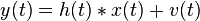
where $*$ denotes convolution and:

$\ x(t)$ is some input signal (unknown) at time $\ t$ .
$\ h(t)$ is the known impulse response of a linear time-invariant system
$\ v(t)$ is some unknown additive noise, independent of $\ x(t)$
$\ y(t)$ is our observed signal

Our goal is to find some $\ g(t)$ so that we can estimate $\ x(t)$ as follows:

$\ \hat{x}(t) = g(t)*y(t)$

where $\ \hat{x}(t)$ is an estimate of $\ x(t)$ that minimizes the mean square error.

The Wiener deconvolution filter provides such a $\ g(t)$ . The filter is most easily described in the frequency domain:

$\ G(f) = \frac{H^*(f)S(f)}{ |H(f)|^2 S(f) + N(f) }$

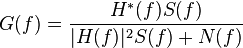
where:

$\ G(f)$ and $\ H(f)$ are the Fourier transforms of $\ g$ and $\ h$ , respectively at frequency $\ f$ .
$\ S(f)$ is the mean power spectral density of the input signal $\ x(t)$
$\ N(f)$ is the mean power spectral density of the noise $\ v(t)$
the superscript ${}^*$ denotes complex conjugation.

The filtering operation may either be carried out in the time-domain, as above, or in the frequency domain:

$\ \hat{X}(f) = G(f)Y(f)$

(where $\ \hat{X}(f)$ is the Fourier transform of $\hat{x}(t)$ ) and then performing an inverse Fourier transform on $\ \hat{X}(f)$ to obtain $\ \hat{x}(t)$ .

Note that in the case of images, the arguments $\ t$ and $\ f$ above become two-dimensional; however the result is the same.

[edit]Interpretation

The operation of the Wiener filter becomes apparent when the filter equation above is rewritten:

$\begin{align} G(f) & = \frac{1}{H(f)} \left[ \frac{ |H(f)|^2 }{ |H(f)|^2 + \frac{N(f)}{S(f)} } \right] \\ & = \frac{1}{H(f)} \left[ \frac{ |H(f)|^2 }{ |H(f)|^2 + \frac{1}{\mathrm{SNR}(f)}} \right]\end{align}$

Here, $\ 1/H(f)$ is the inverse of the original system, and 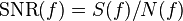$\ \mathrm{SNR}(f) = S(f)/N(f)$ is the signal-to-noise ratio. When there is zero noise (i.e. infinite signal-to-noise), the term inside the square brackets equals 1, which means that the Wiener filter is simply the inverse of the system, as we might expect. However, as the noise at certain frequencies increases, the signal-to-noise ratio drops, so the term inside the square brackets also drops. This means that the Wiener filter attenuates frequencies dependent on their signal-to-noise ratio.

The Wiener filter equation above requires us to know the spectral content of a typical image, and also that of the noise. Often, we do not have access to these exact quantities, but we may be in a situation where good estimates can be made. For instance, in the case of photographic images, the signal (the original image) typically has strong low frequencies and weak high frequencies, and in many cases the noise content will be relatively flat with frequency.

[edit]Derivation

As mentioned above, we want to produce an estimate of the original signal that minimizes the mean square error, which may be expressed:

$\ \epsilon(f) = \mathbb{E} \left| X(f) - \hat{X}(f) \right|^2$

where $\ \mathbb{E}$ denotes expectation.

If we substitute in the expression for $\ \hat{X}(f)$ , the above can be rearranged to

$\begin{align} \epsilon(f) & = \mathbb{E} \left| X(f) - G(f)Y(f) \right|^2 \\ & = \mathbb{E} \left| X(f) - G(f) \left[ H(f)X(f) + V(f) \right] \right|^2 \\ & = \mathbb{E} \big| \left[ 1 - G(f)H(f) \right] X(f) - G(f)V(f) \big|^2\end{align}$

If we expand the quadratic, we get the following:

$\begin{align} \epsilon(f) & = \Big[ 1-G(f)H(f) \Big] \Big[ 1-G(f)H(f) \Big]^*\, \mathbb{E}|X(f)|^2 \\ & {} - \Big[ 1-G(f)H(f) \Big] G^*(f)\, \mathbb{E}\Big\{X(f)V^*(f)\Big\} \\ & {} - G(f) \Big[ 1-G(f)H(f) \Big]^*\, \mathbb{E}\Big\{V(f)X^*(f)\Big\} \\ & {} + G(f) G^*(f)\, \mathbb{E}|V(f)|^2\end{align}$

However, we are assuming that the noise is independent of the signal, therefore:

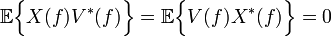
$\ \mathbb{E}\Big\{X(f)V^*(f)\Big\} = \mathbb{E}\Big\{V(f)X^*(f)\Big\} = 0$

Also, we are defining the power spectral densities as follows:

$\ S(f) = \mathbb{E}|X(f)|^2$

$\ N(f) = \mathbb{E}|V(f)|^2$

Therefore, we have:

$\begin{align} \epsilon(f) & = \Big[ 1-G(f)H(f) \Big]\Big[ 1-G(f)H(f) \Big]^* S(f) \\ & {} + G(f)G^*(f)N(f)\end{align}$

To find the minimum error value, we differentiate with respect to $\ G(f)$ and set equal to zero. As this is a complex value, $\ G^*(f)$ acts as a constant.

$\ \frac{d\epsilon(f)}{dG(f)} = G^*(f)N(f) - H(f)\Big[1 - G(f)H(f)\Big]^* S(f) = 0$

This final equality can be rearranged to give the Wiener filter.

[edit]See also

Wikimedia Commons has media related to: An example of Wiener deconvolution on motion blured image (and source codes in MATLAB/GNU Octave).

[edit]References

Rafael Gonzalez, Richard Woods, and Steven Eddins. Digital Image Processing Using Matlab. Prentice Hall, 2003.

[edit]External links

来源：http://en.wikipedia.org/wiki/Wiener_deconvolution

alaclp

关注

2
点赞
踩
9

收藏

觉得还不错? 一键收藏
0
评论
Wiener反卷积方法

Wiener deconvolutionFrom Wikipedia, the free encyclopediaFrom left: Original image, blurred image, image deblurred using Wiener deconvolution.In mathematics, Wiener
复制链接

扫一扫