7、代价聚合Python

最新推荐文章于 2023-08-24 11:24:19 发布

机器人涮火锅

最新推荐文章于 2023-08-24 11:24:19 发布

阅读量954

点赞数 5

分类专栏：人工智能文章标签： python 人工智能

本文链接：https://blog.csdn.net/baidu_39231810/article/details/128633138

版权

人工智能专栏收录该内容

15 篇文章 22 订阅

订阅专栏

文章目录

1、代价聚合理论实现
2、代价聚合实现代码

代价聚合的根本目的是让代价值能够准确的反映像素之间的相关性。匹配代价的计算往往只会考虑局部信息，通过两个像素邻域内一定大小的窗口内的像素信息来计算代价值，这很容易受到影像噪声、弱纹理或重复纹理的影响。而代价聚合则是建立邻接像素之间的联系，以一定的准则，来对代价矩阵进行优化。每个像素在某个视差下的新代价值都会根据其相邻像素在同一视差值或者附近视差值下的代价值来重新计算。
实际上代价聚合类似于一种视差传播步骤，信噪比高的区域匹配效果好，初始代价能够很好的反映相关性，可以更准确的得到最优视差值，通过代价聚合传播至信噪比低、匹配效果不好的区域，最终使所有影像的代价值都能够准确反映真实相关性。常用的代价聚合方法有扫描线法、动态规划法、SGM算法中的路径聚合法等。

1、代价聚合理论实现

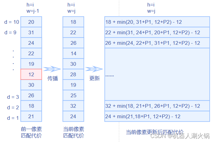
SGM算法提出了代价聚合的想法，就是把像素所有视差下的匹配代价进行像素周围所有路径的一维聚合，得到各个路径下的路径代价，然后将所有路径代价相加得到该像素聚合后的匹配代价值。像素p沿着某条路径r的路径代价计算方法如公式4所示：
$L_r(p,d) = C(p,d) + min\left\{ \begin{matrix} L_r(p-r,d) \\ L_r(p-r,d-1) + P_1 \\ L_r(p-r,d+1) + P_1 \\ \mathop{min}\limits_{i} L_r(p-r,i) + P_2 \end{matrix} \right\} - \mathop{min}\limits_{i}L_r(p-r,i)$

$L_r(p-r,d)$ 表示路径中前一个像素视差为d的代价值
$L_r(p-r,d-1)$ 表示路径中前一个像素视差为d-1时的代价值
$L_r(p-r,d+1)$ 表示路径中前一个像素视差的d+1时的代价值
$minL_r(p-r,i)$ 表示路径中前一个像素所有代价的最小值
$P_1$ 为惩罚项，自己设置
$P_2$ 为惩罚项，自己设置， $P_2$ 一般远大于 $P_1$

其中上式的计算图示如下：
在这里插入图片描述
算法实现关键步骤：

2、代价聚合实现代码

import time
import cv2
import numpy as np
from comput_cost import Compute_Costs

# ========================================================= #

class Aggregate_Cost(object):
    def __init__(self,P1, P2):
        
        self.P1       = P1
        self.P2       = P2


        self.paths = {}
        self.paths['T']  = ( 0,-1)   # 上
        # self.paths['LT'] = (-1,-1)   # 上左
        self.paths['B']  = ( 1, 0)   # 下
        # self.paths['RB'] = ( 1, 1)   # 下右
        self.paths['L']  = ( 0, 1)   # 左
        #self.paths['RT'] = ( 1,-1)   # 右上
        self.paths['R']  = (-1, 0)   # 右
        #self.paths['LB'] = (-1, 1)   # 左下
        
        self.effective_paths = [(self.paths['T'],  self.paths['B']), 
                                #(self.paths['LT'], self.paths['RB']),
                                (self.paths['L'],  self.paths['R']),
                                #(self.paths['RT'], self.paths['LB'])
                                ] 

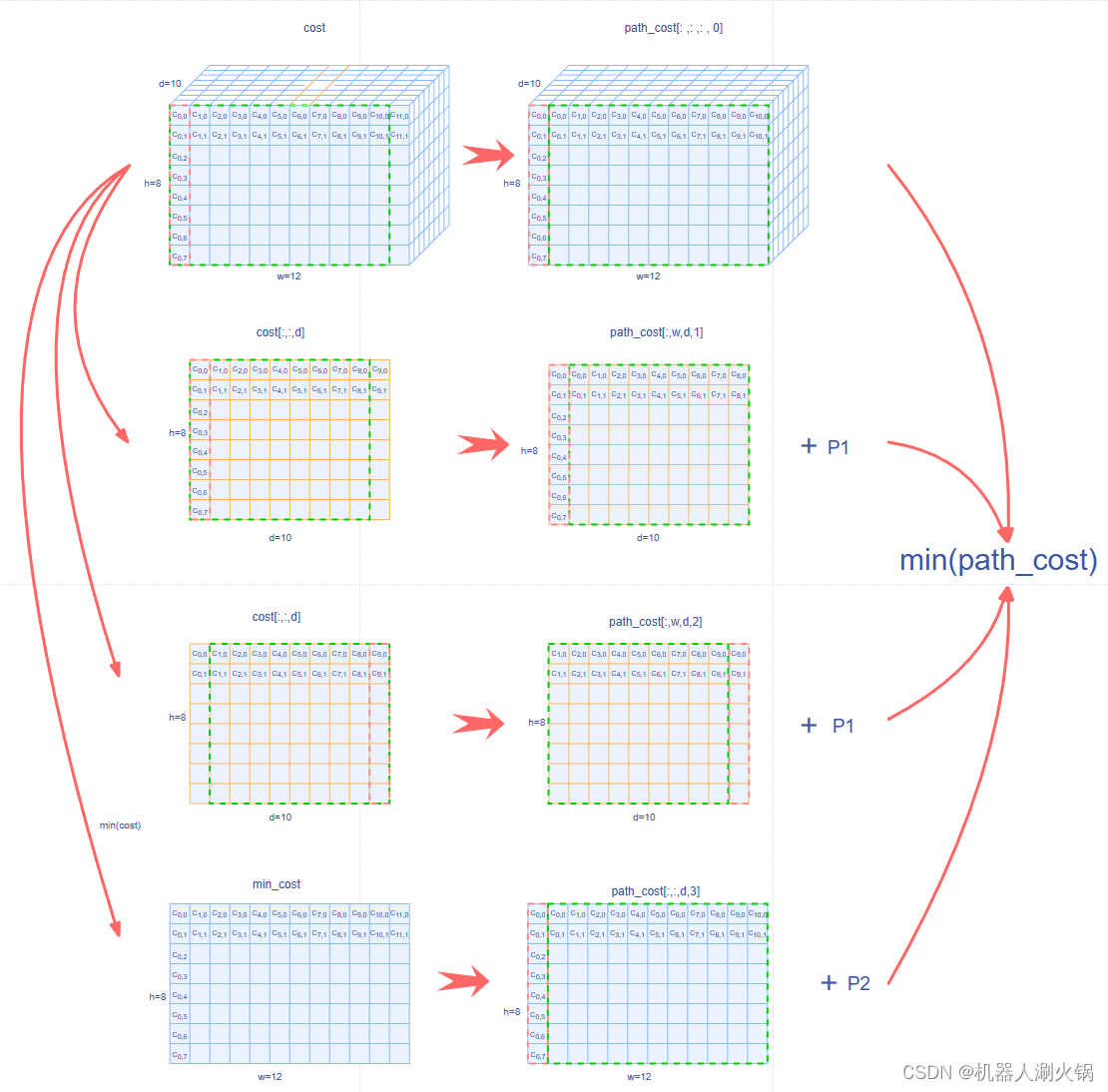
    def get_path_cost(self, cost, path_cost, minimum_cost, flag):
        h, w, d = cost.shape

        if flag == 0:
            path_cost[:,0,:,0] = cost[:,0,:]
            path_cost[:,1:w,:,0] = cost[:,0:w-1,:]

            path_cost[:,:,0,1] =  path_cost[:,:,0,0]
            path_cost[:,:,1:d,1] =  path_cost[:,:,0:d-1,0] + self.P1

            path_cost[:,:,-1,2] =  path_cost[:,:,-1,0]
            path_cost[:,:,0:d-1,2] =  path_cost[:,:,1:d,0] + self.P1

            min_cost = np.min(path_cost[:,:,:,0], axis=2)
            path_cost[:,:,:,3] = np.expand_dims(min_cost,2).repeat(d,axis=2) + self.P2

        elif flag == 1:
            path_cost[0,:,:,0] = cost[0,:,:]
            path_cost[1:h,:,:,0] = cost[0:h-1,:,:]

            path_cost[:,:,0,1] =  path_cost[:,:,0,0]
            path_cost[:,:,1:d,1] =  path_cost[:,:,0:d-1,0] + self.P1

            path_cost[:,:,-1,2] =  path_cost[:,:,-1,0]
            path_cost[:,:,0:d-1,2] =  path_cost[:,:,1:d,0] + self.P1

            min_cost = np.min(path_cost[:,:,:,0], axis=2)
            path_cost[:,:,:,3] = np.expand_dims(min_cost,2).repeat(d,axis=2) + self.P2

        minimum_cost_path = cost + np.min(path_cost, axis=3) - minimum_cost
        return minimum_cost_path

    #     # 代价聚合
    def costs_aggregate(self,costs):
        height = costs.shape[0]
        width = costs.shape[1]
        disparities = costs.shape[2]

        minimum_cost = np.min(costs, axis=2)
        minimum_cost = np.expand_dims(minimum_cost,2).repeat(disparities,axis=2)

        path_cost = np.zeros(shape=(height, width, disparities, 4), dtype=costs.dtype)
        
        aggregation_volume=np.zeros((height, width, disparities,len(self.paths)),dtype=np.int64)

        path_id = 0
        for path in self.effective_paths:
            dawn = time.time()
            
            if path[0] == self.paths['L']:
                left = costs
                right = np.flip(costs,axis=1)

                main_aggregation = self.get_path_cost(left,path_cost, minimum_cost,flag=0)
                opposite_aggregation = np.flip(self.get_path_cost(right,path_cost, minimum_cost,flag=0), axis=1)
    
            if path[0] == self.paths['T']:
                top = costs
                button = np.flip(costs,axis=0)

                main_aggregation = self.get_path_cost(top, path_cost, minimum_cost, flag=1)
                opposite_aggregation = np.flip(self.get_path_cost(button, path_cost, minimum_cost,flag=1), axis=1)
    
         
    
            aggregation_volume[:, :, :, path_id] = main_aggregation
            aggregation_volume[:, :, :, path_id + 1] = opposite_aggregation
            path_id = path_id + 2
    
            dusk = time.time()
            print('\t(aggregation path{:} in {:.2f}s)'.format(path_id, dusk - dawn))
        
        volume = np.sum(aggregation_volume, axis=3)
        disparity_map = np.argmin(volume, axis=2)
        return disparity_map


if __name__ == '__main__':

    imgL=np.asanyarray(cv2.imread('./data/test/left_000.png',0),dtype=np.int64)
    imgR=np.asanyarray(cv2.imread('./data/test/right_000.png',0),dtype=np.int64)

    tic1=time.time()

    maxDisparity=12 # 最大视差，也就是搜索范围，搜索范围越大耗时越长
                    # 可以根据需求的有效测距范围来大致计算出最小和最大视差

    window_size = 5               # 滑动窗口大小，窗口越大匹配成功难度越高
    radius=np.int64(window_size/2)# 窗口大小的一半向下取整，比如用来衡量窗口左上角与窗口中点的距离的x与y坐标
    lamda = 20

    P1 = 10
    P2 = 75
    bsize = 3

    h,w = imgL.shape[0:2]

    compute_costs = Compute_Costs(h,w,maxDisparity, window_size, radius, lamda)
    aggregate_cost = Aggregate_Cost(P1, P2)
    # 代价计算
    costs = compute_costs.AD(imgL, imgR)
    #costs = compute_costs.SAD(imgL, imgR)
    #costs = compute_costs.Census(imgL, imgR)
    #costs = compute_costs.CensusAD(imgL, imgR)
    # 代价聚合
    disparity_map = aggregate_cost.costs_aggregate(costs)
    #disparity = cv2.medianBlur(np.uint8(disparity_map), bsize)



    # 生成深度图（颜色图）
    dis_color = disparity_map
    dis_color = cv2.normalize(dis_color, None, alpha=0, beta=255, norm_type=cv2.NORM_MINMAX, dtype=cv2.CV_8U)
    dis_color = cv2.applyColorMap(dis_color, 2)

    print('总用时:{:.2f}s'.format(time.time()-tic1))

    cv2.imshow('dispmap',dis_color)
    cv2.waitKey()

机器人涮火锅

关注

5
点赞
踩
23

收藏

觉得还不错? 一键收藏
打赏
2
评论
7、代价聚合Python

代价聚合的根本目的是让代价值能够准确的反映像素之间的相关性。匹配代价的计算往往只会考虑局部信息，通过两个像素邻域内一定大小的窗口内的像素信息来计算代价值，这很容易受到影像噪声、弱纹理或重复纹理的影响。而代价聚合则是建立邻接像素之间的联系，以一定的准则，来对代价矩阵进行优化。每个像素在某个视差下的新代价值都会根据其相邻像素在同一视差值或者附近视差值下的代价值来重新计算。
复制链接

扫一扫