python实现之多元函数作图

多元函数的本质是一种关系，是两个集合间一种确定的对应关系。多元函数是后续人工智能的基础，先可视化呈现，后续再学习一下求导。

设D为一个非空的n 元有序数组的集合， f为某一确定的对应规则。若对于每一个有序数组 ( x1,x2,…,xn)∈D，通过对应规则f，都有唯一确定的实数y与之对应，则称对应规则f为定义在D上的n元函数。

记为y=f(x1,x2,…,xn) 其中 ( x1,x2,…,xn)∈D。变量x1,x2,…,xn称为自变量，y称为因变量。

当n=1时，为一元函数，记为y=f(x),x∈D，当n=2时，为二元函数，记为z=f(x,y),(x,y)∈D。二元及以上的函数统称为多元函数。 

#!/usr/bin/env python
# -*- coding: UTF-8 -*-
#                     _ooOoo_
#                   o8888888o
#                    88" . "88
#                 ( | -  _  - | )
#                     O\ = /O
#                 ____/`---'\____
#                  .' \\| |// `.
#                 / \\|||:|||// \
#               / _|||||-:- |||||- \
#                | | \\\ - /// | |
#              | \_| ''\---/'' | _/ |
#               \ .-\__ `-` ___/-. /
#            ___`. .' /--.--\ `. . __
#         ."" '< `.___\_<|>_/___.' >'"".
#       | | : `- \`.;`\  _ /`;.`/ - ` : | |
#          \ \ `-. \_ __\ /__ _/ .-` / /
#      ==`-.____`-.___\_____/___.-`____.-'==
#                     `=---='
'''
@Project ：pythonalgorithms 
@File ：multivariatefunc.py
@Author ：不胜人生一场醉@Date ：2021/8/6 23:59 
'''
import numpy as np
# mpl_toolkits是matplotlib官方的工具包 mplot3d是用来画三维图像的工具包
from mpl_toolkits.mplot3d import Axes3D
from matplotlib import pyplot as plt
from matplotlib.ticker import LinearLocator, FormatStrFormatter

# 绘制z=x^2+y^2的3D图
# 创建一个图像窗口
fig = plt.figure()
# 在图像窗口添加3d坐标轴
ax = Axes3D(fig)
# 使用np.arange定义 x:范围(-10,10);间距为0.1
x = np.arange(-10, 10, 0.1)
# 使用np.arange定义 y:范围(-10,10);间距为0.1
y = np.arange(-10, 10, 0.1)
# 创建x-y平面网络
x, y = np.meshgrid(x, y)
# 定义函数z=x^2+y^2
z = x * x + y * y
# 将函数显示为3d  rstride 和 cstride 代表 row(行)和column(列)的跨度 cmap为色图分类
ax.plot_surface(x, y, z, rstride=1, cstride=1, cmap='rainbow')
plt.show()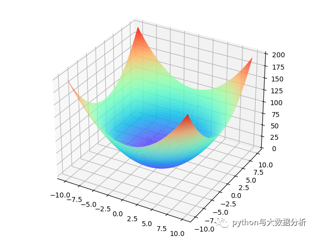

# 绘制z=sin(sqrt(x^2+y^2))的3D图
fig = plt.figure()
ax = Axes3D(fig)  # 设置图像为三维格式
x = np.arange(-10, 10, 0.1)  # x的范围
y = np.arange(-10, 10, 0.1)  # y的范围
x, y = np.meshgrid(x, y)  # 绘制网格
z = np.sin(np.sqrt(x*x+y*y))
ax.plot_surface(x, y, z, rstride=1, cstride=1, cmap='rainbow')
plt.show()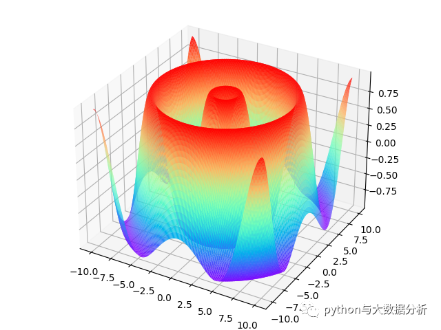

# 绘制z=sin(x)^2+sin(y)^2的3D图
fig = plt.figure()
ax = Axes3D(fig)  # 设置图像为三维格式
x = np.arange(-10, 10, 0.1)  # x的范围
y = np.arange(-10, 10, 0.1)  # y的范围
x, y = np.meshgrid(x, y)  # 绘制网格
z = np.sin(x) * np.sin(y)
ax.plot_surface(x, y, z, rstride=1, cstride=1, cmap='rainbow')
plt.show()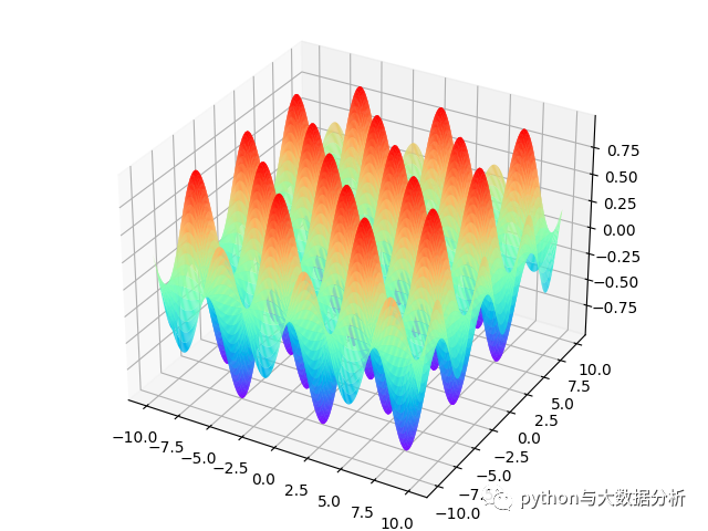

# 绘制z=x*y的3D图
fig = plt.figure()
ax = Axes3D(fig)  # 设置图像为三维格式
x = np.arange(-10, 10, 0.1)  # x的范围
y = np.arange(-10, 10, 0.1)  # y的范围
x, y = np.meshgrid(x, y)  # 绘制网格
z = x * y
ax.plot_surface(x, y, z, rstride=1, cstride=1, cmap='rainbow')
plt.show()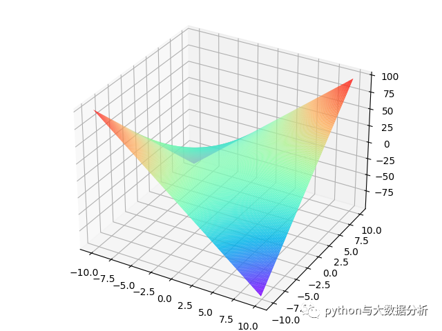

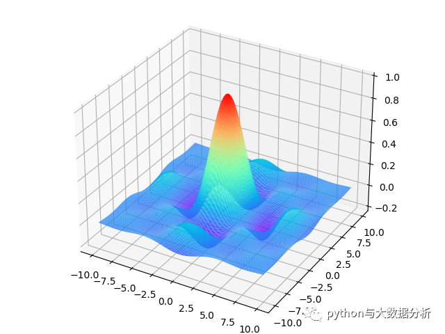
# 绘制z=sin(x)*sin(y)/x/y的3D图
fig = plt.figure()
ax = Axes3D(fig)  # 设置图像为三维格式
x = np.arange(-10, 10, 0.1)  # x的范围
y = np.arange(-10, 10, 0.1)  # y的范围
x, y = np.meshgrid(x, y)  # 绘制网格
z = np.sin(x) * np.sin(y) / (x * y)
ax.plot_surface(x, y, z, rstride=1, cstride=1, cmap='rainbow')
plt.show()

# 绘制z=sin(x)*sin(y)+cos(x)*cos(y)的3D图
fig = plt.figure()
ax = Axes3D(fig)  # 设置图像为三维格式
x = np.arange(-10, 10, 0.1)  # x的范围
y = np.arange(-10, 10, 0.1)  # y的范围
x, y = np.meshgrid(x, y)  # 绘制网格
z = np.sin(x) * np.sin(y) + np.cos(x) * np.cos(y)
ax.plot_surface(x, y, z, rstride=1, cstride=1, cmap='rainbow')
plt.show()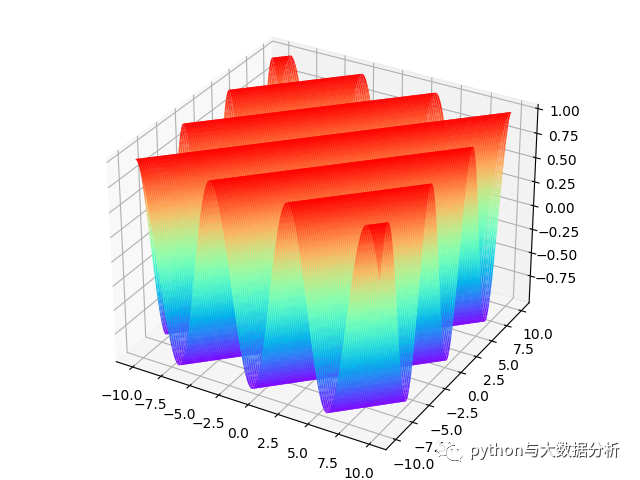

# 绘制z=-(x*y)/e^(x^2+y^2)的3D图
fig = plt.figure()
ax = Axes3D(fig)
x = np.arange(-2, 2, 0.01)
y = np.arange(-2, 2, 0.01)
x, y = np.meshgrid(x, y)
r = - x * y
z = r / np.e ** (x ** 2 + y ** 2)
surf = ax.plot_surface(x, y, z, rstride=1, cstride=1, cmap='rainbow', linewidth=0, antialiased=False)
ax.set_zlim(-1.01, 1.01)
ax.zaxis.set_major_locator(LinearLocator(10))
ax.zaxis.set_major_formatter(FormatStrFormatter('%.02f'))
fig.colorbar(surf, shrink=0.5, aspect=5)
plt.show()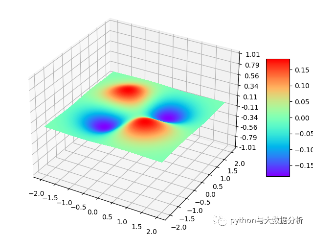

# 绘制z=-(x*y)/e^(x^2+y^2)的3D图
fig = plt.figure()
ax = Axes3D(fig)
x = np.arange(-2, 2, 0.01)
y = np.arange(-2, 2, 0.01)
x, y = np.meshgrid(x, y)
r = - x * y
z = r / np.e ** (x ** 2 + y ** 2)
surf = ax.plot_surface(x, y, z, rstride=1, cstride=1, cmap='rainbow', linewidth=0, antialiased=False)
ax.set_zlim(-1.01, 1.01)
ax.zaxis.set_major_locator(LinearLocator(10))
ax.zaxis.set_major_formatter(FormatStrFormatter('%.02f'))
# 在xy 平面添加等高线， contourf会对区间进行填充
ax.contourf(x, y, z, zdir="z", offset=-2, cmap='rainbow')
fig.colorbar(surf, shrink=0.5, aspect=5)
plt.show()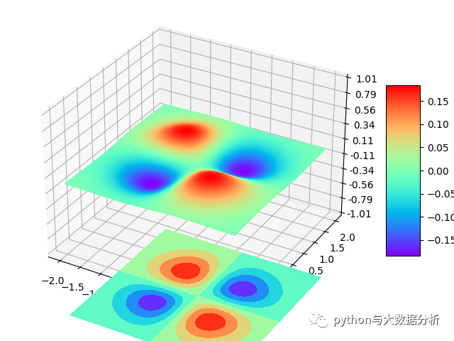

原创不易,转载请注明！请多多关注，谢谢！