基于局部统计的可变阈值处理&使用移动平均的图像阈值处理

 

前言

尽管在前面的介绍中我们似乎已经实现了图像的阈值处理，但事实并非如此，因为在图像处理时依然会遇到之前的方法无法解决的阈值处理问题。这里简单介绍两种改进图像阈值处理的方法，分别是基于局部统计的可变阈值处理和使用移动平均的图像阈值处理。

 

一、基于局部统计的可变阈值处理

在前面的全局阈值处理中我们曾经使用过一幅酵母细胞的图像进行阈值处理，实际上在那幅图像中共有三个比较明显的灰度级，分别是背景灰度级、细胞质灰度级和细胞核灰度级。无论利用之前介绍的何种方法，我们都不能实现将它们三个完全区别开来的阈值处理，而基于局部统计的可变阈值处理就可以实现这一目的。在进行局部阈值处理时，需要用到图像中每一点的邻域中像素的标准差和均值。要计算局部标准差，matlab中有现成的函数stdfilt，语法为：

                                                                                                                     g=stdfilt(f,nhood)

其中f为输入图像，nhood为0和1组成的数组，其中的非零元素指定用于计算局部标准差所用的邻域。nhood默认为ones(3)

计算局部均值时我们可以使用自定义函数localmean，其具体的实现代码如下：

function mean=localmean(f,nhood)
if nargin==1
    nhood=ones(3)/9;
else
    nhood=nhood/sum(nhood(:));
end
mean=imfilter(tofloat(f),nhood,'replicate');
end

因此基于局部统计的可变阈值T=a*δ（xy）+b*m(xy)

冈萨雷斯的书上介绍说，我们在使用这个方法时可以采用全局阈值并引入布尔运算对阈值处理添加权重，因此最后得到的g应该为：

g(x,y)=1,f(x,y)> a*δ（xy）AND f(x,y)>b*m

g(x,y)=0,others

为了更简便的实现基于局部统计的可变阈值处理，我们采用自定义函数localthresh，其代码如下：

function g=localthresh(f,nhood,a,b,meantype)
f=tofloat(f);
SIG=stdfilt(f,nhood);
if nargin==5 && strcmp(meantype,'global')
    MEAN=mean2(f);
else
    MEAN=localmean(f,nhood);
end
g=(f>a*SIG) & (f>b*MEAN);
end

二、代码示例

对之前采用全局阈值处理的酵母细胞重新进行处理，并对比两种处理方式之间的差异。

具体代码如下：

I1=imread('cell.tif');
I1=tofloat(I1);%改变图像类型
[Tf SMf]=graythresh(I1);%先对图像直接使用Otsu方法
I2=im2bw(I1,Tf);
figure(2)
subplot(221),imshow(I1),title('原图');
subplot(222),imshow(I2),title('使用Otsu方法直接进行分割');
g=localthresh(I1,ones(3),30,1.5,'global');%利用局部标准差的方法对图像进行分割
SIG=stdfilt(I1,ones(3));
subplot(223),imshow(SIG,[ ]),title('局部标准差图像');
subplot(224),imshow(g),title('局部阈值分割处理图像');

三、结果展示及分析

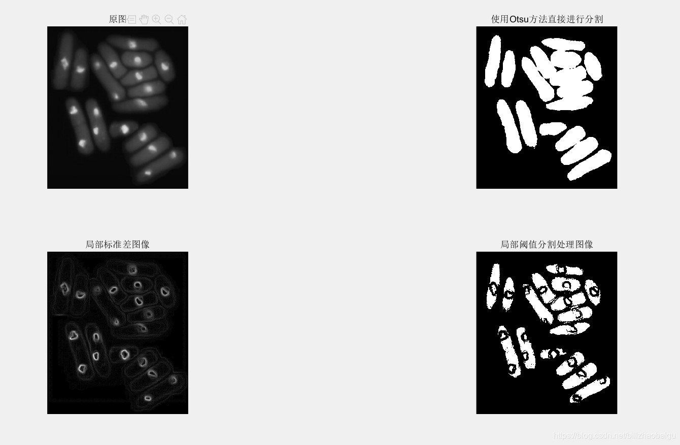
可以看到采用局部统计的可变阈值处理的方式进行图像分割是十分有效的。不仅实现了细胞的单个分离，还成功地将细胞核和细胞质进行了区分，这比利用Otsu的全局阈值处理方法要优越得多。

 

四、使用移动平均的图像阈值处理

在使用文本处理时，非常常用的方法是沿一幅图像的扫描线来计算移动平均。针对移动平均这里我并没能很好的掌握原理，根据冈萨雷斯书的指导，在使用该方法时会引入一个“movingthresh”的自定义函数，可以直接实现移动平均的图像阈值处理。

具体的代码为：

function g = movingthresh(f, n, K)  
%MOVINGTHRESH Image segmentation using a moving average threshold.  
%   G = MOVINGTHRESH(F, n, K) segments image F by thresholding its  
%   intensities based on the moving average of the intensities along  
%   individual rows of the image. The average at pixel k is formed  
%   by averaging the intensities of that pixel and its n ? 1  
%   preceding neighbors. To reduce shading bias, the scanning is  
%   done in a zig-zag manner, treating the pixels as if they were a  
%   1-D, continuous stream. If the value of the image at a point  
%   exceeds K percent of the value of the running average at that  
%   point, a 1 is output in that location in G. Otherwise a 0 is  
%   output. At the end of the procedure, G is thus the thresholded  
%    (segmented) image. K must be a scalar in the range [0, 1].  
 
% Preliminaries. 
% || means or operator;rem(n,1) means the residual of n/1
f = tofloat(f);  
[M, N] = size(f);  
if (n < 1) || (rem(n, 1) ~= 0)  
   error('n must be an integer >= 1.')  
end  
if K < 0 || K > 1  
   error('K must be a fraction in the range [0, 1].')  
end  
 
% Flip every other row of f to produce the equivalent of a zig-zag scanning pattern. Convert image to a vector.  
f(2:2:end, :) = fliplr(f(2:2:end, :));  %fliplr realize the overturn of the vector 
f = f'; % Still a matrix.  
f = f(:)'; % Convert to row vector for use in function filter.  
 
% Compute the moving average.  
maf = ones(1, n)/n; % The 1-D moving average filter.  
ma = filter(maf, 1, f); % Computation of moving average.  
 
% Perform thresholding.  
g = (f > K * ma);  
 
% Go back to image format (indexed subscripts).  
g = reshape(g, N, M)';  
% Flip alternate(交替的) rows back.  
g(2:2:end, :) = fliplr(g(2:2:end, :));  

五、代码示例

我们针对两幅被不同噪声污染的文字图像进行阈值处理来观察该方法的处理效果。处理的目的是想要提取出文字部分。

I1=imread('paper.tif');
T1=graythresh(I1);
I2=im2bw(I1,T1);
I3=movingthresh(I1,20,0.5);
subplot(231),imshow(I1),title('原图');
subplot(232),imshow(I2),title('使用Otsu的处理结果');
subplot(233),imshow(I3),title('使用移动平均的处理结果');

I4=imread('paper1.tif');
T2=graythresh(I4);
I5=im2bw(I4,T2);
I6=movingthresh(I4,20,0.5);
subplot(234),imshow(I4),title('原图');
subplot(235),imshow(I5),title('使用Otsu的处理结果');
subplot(236),imshow(I6),title('使用移动平均的处理结果');

六、结果展示及分析

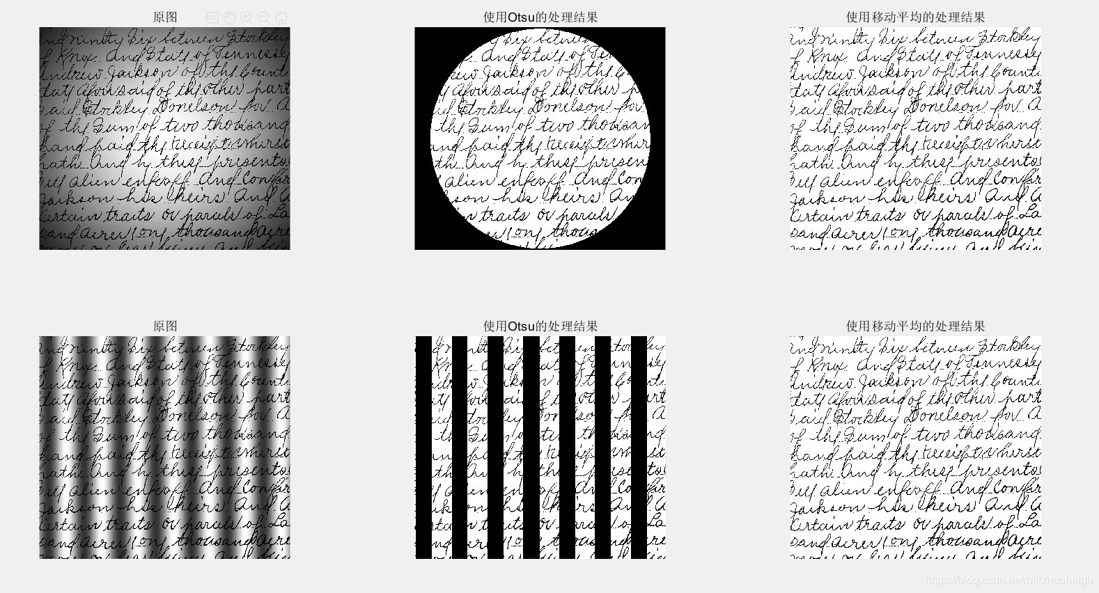
可以看到无论是被斑点遮光污染还是被正弦函数污染的文字图像，在使用过移动平均的图像阈值处理之后都可以得到非常好的图像处理效果，噪声能够被完全清除，这是Otsu方法不能够实现的。在代码中我们规定窗口的宽度为20，这是因为平均宽度为4个像素，理想的窗口宽度是平均笔画宽度的5倍，因此定义为20.而令K=0.5或其他值对结果并不会造成特别大的区别。实际上，这种方法对n和K的值要求并不严格，具有很好的稳定性。当输入图像为手写文本图像时，使用基于移动平均的图像阈值处理往往会得到很好的处理效果。 

---