PyTorch进行CIFAR-10图像分类

本节将通过一个实战案例来详细介绍如何使用PyTorch进行深度学习模型的开发。我们将使用CIFAR-10图像数据集来训练一个卷积神经网络。

神经网络训练的一般步骤如图5-3所示。

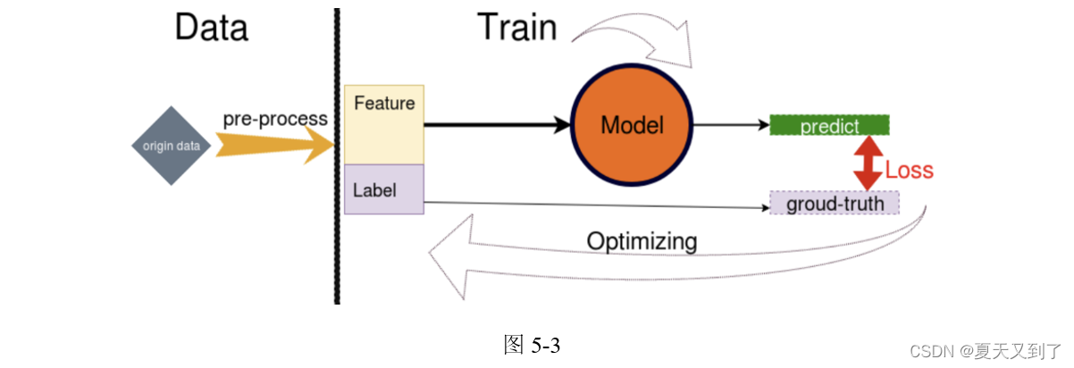
（1）加载数据集，并做预处理。

（2）预处理后的数据分为Feature和Label两部分，Feature 送到模型里面，Label被当作ground-truth。

（3）Model接收Feature作为Input，并通过一系列运算，向外输出 predict。

（4）建立一个损失函数 Loss，Loss 的函数值是为了表示 predict 与 ground-truth 之间的差距。

（5）建立 Optimizer 优化器，优化的目标就是 Loss 函数，让它的取值尽可能最小，Loss越小代表 Model 预测的准确率越高。

（6）Optimizer 优化过程中，Model 根据规则改变自身参数的权重，这是一个反复循环和持续的过程，直到Loss值趋于稳定，不能再取得更小的值。

数据集的加载可以自行编写代码，但如果是基于学习目的的话，那么把精力放在编写这个步骤的代码上面会让人十分无聊，好在PyTorch 提供了非常方便的包torchvision。torchvison提供了dataloader来加载常见的MNIST、CIFAR-10、ImageNet 等数据集，也提供了transform对图像进行变换、正则化和可视化。

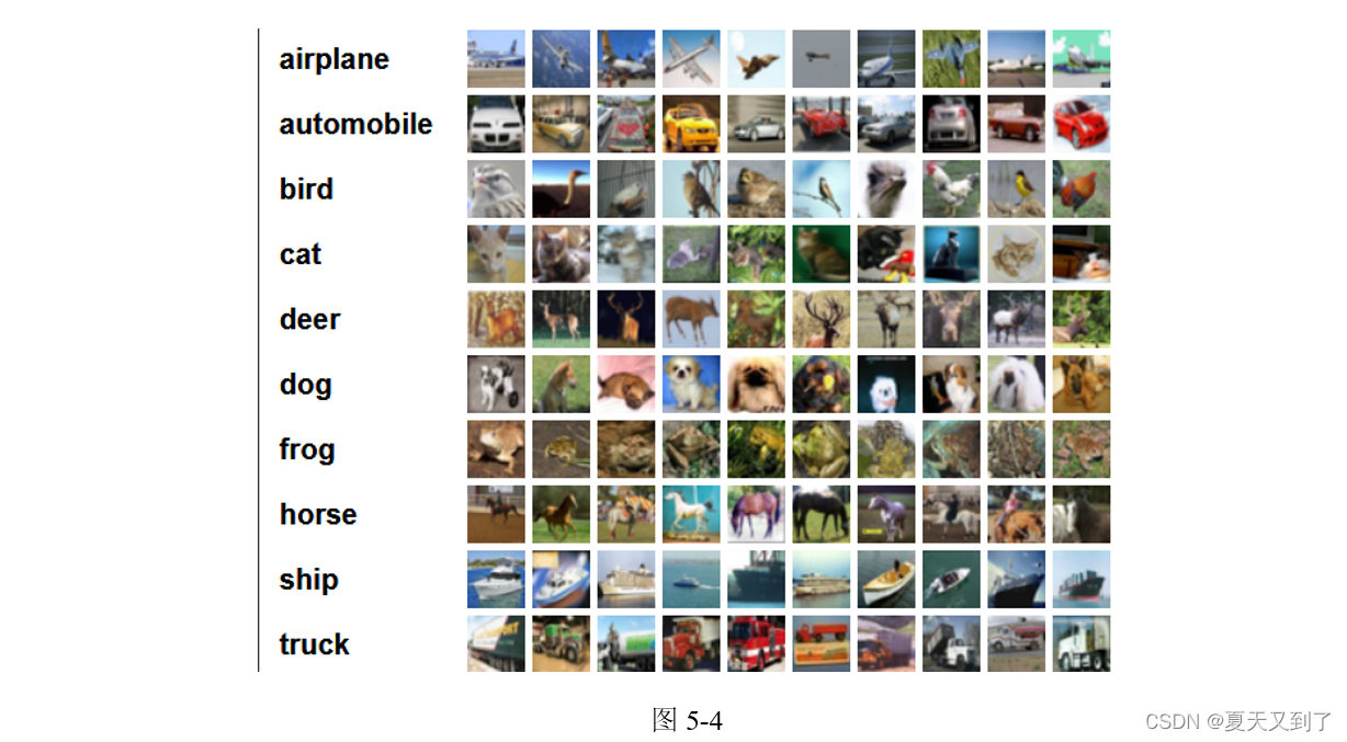
在本项目中，我们的目的是用 PyTorch 创建基于 CIFAR-10 数据集的图像分类器。CIFAR-10图像数据集共有60 000幅彩色图像，这些图像是32×32的，分为10个类，分别是airplane、automobile、bird、cat等，每类6 000幅图，如图5-4所示。这里面有50 000幅训练图像，10 000幅测试图像。

首先，加载数据并进行预处理。我们将使用torchvision包来下载CIFAR-10数据集，并使用transforms模块对数据进行预处理。主要用来进行数据增强，为了防止训练出现过拟合，通常在小型数据集上，通过随机翻转图片、随机调整图片的亮度来增加训练时数据集的容量。但是，测试的时候，并不需要对数据进行增强。运行代码后，会自动下载数据集。

接下来，定义卷积神经网络模型。在这个网络模型中，我们使用nn.Module来定义网络模型，然后在__init__方法中定义网络的层，最后在forward方法中定义网络的前向传播过程。在PyTorch中可以通过继承nn.Module来自定义神经网络，在init()中设定结构，在forward()中设定前向传播的流程。因为PyTorch可以自动计算梯度，所以不需要特别定义反向传播。

定义好神经网络模型后，还需要定义损失函数（Loss）和优化器（Optimizer）。在这里采用 cross-entropy-loss函数作为损失函数，采用 Adam 作为优化器，当然SGD也可以。

一切准备就绪后，开始训练网络，这里训练10次（可以增加训练次数，提高准确率）。在训练过程中，首先通过网络进行前向传播得到输出，然后计算输出与真实标签的损失，接着通过后向传播计算梯度，最后使用优化器更新模型参数。训练完成后，我们需要在测试集上测试网络的性能。这可以让我们了解模型在未见过的数据上的表现如何，以评估其泛化能力。

完整代码如下：

#############cifar-10-pytorch.py####################
import torch
import torch.nn as nn
import torch.nn.functional as F
from torch.autograd import Variable
import torch
import torchvision
import torchvision.transforms as transforms
import torch.optim as optim

# torchvision输出的是PILImage，值的范围是[0, 1]
# 我们将其转换为张量数据，并归一化为[-1, 1]
transform = transforms.Compose([transforms.ToTensor(),
                                transforms.Normalize(mean=(0.5, 0.5, 0.5),
                                                     std=(0.5, 0.5, 0.5)),
                                ])

# 训练集，将相对目录./data下的cifar-10-batches-py文件夹中的全部数据
# （50 000幅图片作为训练数据）加载到内存中
# 若download为True，则自动从网上下载数据并解压
trainset = torchvision.datasets.CIFAR10(root='./data', train=True,
                                        download=True, transform=transform)

# 将训练集的50 000幅图片划分成12 500份，每份4幅图，用于mini-batch输入
# shffule=True在表示不同批次的数据遍历时，打乱顺序。num_workers=2表示使用两个子进程来加载数据
trainloader = torch.utils.data.DataLoader(trainset, batch_size=4,
                                          shuffle=False, num_workers=2)

classes = ('plane', 'car', 'bird', 'cat',
           'deer', 'dog', 'frog', 'horse', 'ship', 'truck')
# 下面的代码只是为了给小伙伴们展示一个图片例子，让大家有个直观感受
# functions to show an image
import matplotlib.pyplot as plt
import numpy as np

# matplotlib inline
def imshow(img):
    img = img / 2 + 0.5  # unnormalize
    npimg = img.numpy()
    plt.imshow(np.transpose(npimg, (1, 2, 0)))
    plt.show()
class Net(nn.Module):
    # 定义Net的初始化函数，这个函数定义了该神经网络的基本结构
    def __init__(self):
        super(Net, self).__init__()
        # 复制并使用Net的父类的初始化方法，即先运行nn.Module的初始化函数
        self.conv1 = nn.Conv2d(3, 6, 5)
        # 定义conv1函数是图像卷积函数：输入为3张特征图
        # 输出为 6幅特征图， 卷积核为5×5的正方形
        self.conv2 = nn.Conv2d(6, 16, 5)
        # 定义conv2函数的是图像卷积函数：输入为6幅特征图，输出为16幅特征图
        # 卷积核为5×5的正方形
        self.fc1 = nn.Linear(16 * 5 * 5, 120)
        # 定义fc1（fullconnect）全连接函数1为线性函数：y = Wx + b
        # 并将16×5×5个节点连接到120个节点上
        self.fc2 = nn.Linear(120, 84)
        # 定义fc2（fullconnect）全连接函数2为线性函数：y = Wx + b
        # 并将120个节点连接到84个节点上
        self.fc3 = nn.Linear(84, 10)
        # 定义fc3（fullconnect）全连接函数3为线性函数：y = Wx + b
        # 并将84个节点连接到10个节点上

    # 定义该神经网络的向前传播函数，该函数必须定义
    # 一旦定义成功，向后传播函数也会自动生成（autograd）
    def forward(self, x):
        x = F.max_pool2d(F.relu(self.conv1(x)), (2, 2))
        # 输入x经过卷积conv1之后，经过激活函数ReLU
        # 使用2×2的窗口进行最大池化，然后更新到x
        x = F.max_pool2d(F.relu(self.conv2(x)), 2)
        # 输入x经过卷积conv2之后，经过激活函数ReLU
        # 使用2×2的窗口进行最大池化，然后更新到x
        x = x.view(-1, self.num_flat_features(x))
        # view函数将张量x变形成一维的向量形式
        # 总特征数并不改变，为接下来的全连接作准备
        x = F.relu(self.fc1(x))
        # 输入x经过全连接1，再经过ReLU激活函数，然后更新x
        x = F.relu(self.fc2(x))
        # 输入x经过全连接2，再经过ReLU激活函数，然后更新x
        x = self.fc3(x)
        # 输入x经过全连接3，然后更新x
        return x

    # 使用num_flat_features函数计算张量x的总特征量
    # 把每个数字都作一个特征，即特征总量
    # 比如x是4×2×2的张量，那么它的特征总量就是16
    def num_flat_features(self, x):
        size = x.size()[1:]
        # 这里为什么要使用[1:]，是因为PyTorch只接受批输入
        # 也就是说一次性输入好几幅图片，那么输入数据张量的维度自然上升到了4维
        # 【1:】让我们把注意力放在后3维上面
        # x.size() 会 return [nSamples, nChannels, Height, Width]。
        # 只需要展开后三项成为一个一维的张量
        num_features = 1
        for s in size:
            num_features *= s
        return num_features
net = Net()
criterion = nn.CrossEntropyLoss()  # 交叉熵损失函数
optimizer = optim.SGD(net.parameters(), lr=0.001, momentum=0.9)
# 使用SGD（随机梯度下降）优化，学习率为0.001，动量为0.9
if __name__ == '__main__':
    for epoch in range(10):
        running_loss = 0.0
        # enumerate(sequence, [start=0])，i是序号，data是数据
        for i, data in enumerate(trainloader, 0):
            inputs, labels = data
            # data的结构是：[4×3×32×32的张量，长度为4的张量]
            inputs, labels = Variable(inputs), Variable(labels)
            # 把input数据从tensor转为variable

            optimizer.zero_grad()
            # 将参数的grad值初始化为0
            # forward + backward + optimize
            outputs = net(inputs)
            loss = criterion(outputs, labels)
            # 将output和labels使用交叉熵计算损失
            loss.backward()  # 反向传播
            optimizer.step()  # 用SGD更新参数

            # 每2000批数据打印一次平均loss值
            running_loss += loss.item()
            # loss本身为Variable类型
            # 要使用data获取其张量，因为其为标量，所以取0 或使用loss.item()
            if i % 2000 == 1999:  # 每2000批打印一次
                print('[%d, %5d] loss: %.3f' % (epoch + 1, i + 1, running_loss / 2000))
                running_loss = 0.0

    print('Finished Training')
    # 测试集，将相对目录./data下的cifar-10-batches-py文件夹中的全部数据
    # （10 000幅图片作为测试数据）加载到内存中
    # 若download为True，则自动从网上下载数据并解压
    testset = torchvision.datasets.CIFAR10(root='./data', train=False,
                                           download=True, transform=transform)

    # 将测试集的10 000幅图片划分成2500份，每份4幅图，用于mini-batch输入
    testloader = torch.utils.data.DataLoader(testset, batch_size=4,
                                             shuffle=False, num_workers=2)
    correct = 0
    total = 0
    with torch.no_grad():
        for data in testloader:
            images, labels = data
            outputs = net(Variable(images))
            # print outputs.data
            # print(outputs.data)
            # print(labels)
            value, predicted = torch.max(outputs.data,
                                         1)
            # outputs.data是一个4x10张量
            # 将每一行的最大的那一列的值和序号各自组成一个一维张量返回
            # 第一个是值的张量，第二个是序号的张量
            # label.size(0) 是一个数
            total += labels.size(0)
            correct += (predicted == labels).sum()
            # 两个一维张量逐行对比，相同的行记为1，不同的行记为0
            # 再利用sum()求总和，得到相同的个数

    print('Accuracy of the network on the 10000 test images: %d %%' % (100 * correct / total))

    class_correct = list(0. for i in range(10))
    class_total = list(0. for i in range(10))
    with torch.no_grad():
        for data in testloader:
            images, labels = data
            outputs = net(images)
            _, predicted = torch.max(outputs, 1)
            c = (predicted == labels).squeeze()
            for i in range(4):
                label = labels[i]
                class_correct[label] += c[i].item()
                class_total[label] += 1
    for i in range(10):
        print('Accuracy of %5s : %2d %%' % (classes[i], 100 * class_correct[i] / class_total[i]))

运行结果如下：

Files already downloaded and verified
Files already downloaded and verified
Files already downloaded and verified
[1,  2000] loss: 2.165
[1,  4000] loss: 1.834
[1,  6000] loss: 1.667
[1,  8000] loss: 1.566
[1, 10000] loss: 1.532
[1, 12000] loss: 1.462
Files already downloaded and verified
Files already downloaded and verified
[2,  2000] loss: 1.403
[2,  4000] loss: 1.380
[2,  6000] loss: 1.325
[2,  8000] loss: 1.281
[2, 10000] loss: 1.304
[2, 12000] loss: 1.262
Files already downloaded and verified
Files already downloaded and verified
[3,  2000] loss: 1.230
[3,  4000] loss: 1.221
[3,  6000] loss: 1.181
[3,  8000] loss: 1.147
[3, 10000] loss: 1.175
[3, 12000] loss: 1.147
Files already downloaded and verified
Files already downloaded and verified
[4,  2000] loss: 1.120
[4,  4000] loss: 1.110
[4,  6000] loss: 1.079
[4,  8000] loss: 1.064
[4, 10000] loss: 1.090
[4, 12000] loss: 1.068
Files already downloaded and verified
Files already downloaded and verified
[5,  2000] loss: 1.039
[5,  4000] loss: 1.030
[5,  6000] loss: 1.009
[5,  8000] loss: 0.990
[5, 10000] loss: 1.021
[5, 12000] loss: 1.007
Files already downloaded and verified
Files already downloaded and verified
[6,  2000] loss: 0.975
[6,  4000] loss: 0.971
[6,  6000] loss: 0.947
[6,  8000] loss: 0.937
[6, 10000] loss: 0.963
[6, 12000] loss: 0.953
Files already downloaded and verified
Files already downloaded and verified
[7,  2000] loss: 0.930
[7,  4000] loss: 0.923
[7,  6000] loss: 0.902
[7,  8000] loss: 0.891
[7, 10000] loss: 0.928
[7, 12000] loss: 0.911
Files already downloaded and verified
Files already downloaded and verified
[8,  2000] loss: 0.881
[8,  4000] loss: 0.890
[8,  6000] loss: 0.864
[8,  8000] loss: 0.868
[8, 10000] loss: 0.896
[8, 12000] loss: 0.875
Files already downloaded and verified
Files already downloaded and verified
[9,  2000] loss: 0.846
[9,  4000] loss: 0.870
[9,  6000] loss: 0.836
[9,  8000] loss: 0.834
[9, 10000] loss: 0.851
[9, 12000] loss: 0.847
Files already downloaded and verified
Files already downloaded and verified
[10,  2000] loss: 0.816
[10,  4000] loss: 0.835
[10,  6000] loss: 0.797
[10,  8000] loss: 0.805
[10, 10000] loss: 0.841
[10, 12000] loss: 0.809
Finished Training
Files already downloaded and verified
Files already downloaded and verified
Files already downloaded and verified
Accuracy of the network on the 10000 test images: 61 %
Files already downloaded and verified
Files already downloaded and verified
Accuracy of plane : 58 %
Accuracy of   car : 72 %
Accuracy of  bird : 41 %
Accuracy of   cat : 51 %
Accuracy of  deer : 55 %
Accuracy of   dog : 44 %
Accuracy of  frog : 66 %
Accuracy of horse : 72 %
Accuracy of  ship : 80 %
Accuracy of truck : 69 %

在这段代码中，我们在整个测试集上测试网络，并打印出网络在测试集上的准确率。通过这种详细且实践性的方式介绍了PyTorch的使用，包括张量操作、自动求导机制、神经网络创建、数据处理、模型训练和测试。我们利用PyTorch从头到尾完成了一个完整的神经网络训练流程，并在 CIFAR-10数据集上测试了网络的性能。在这个过程中，我们深入了解了PyTorch提供的强大功能。

本文节选自《PyTorch深度学习与企业级项目实战》，获出版社和作者授权发布。