《Keras | 莫烦》learning notes

bryant_meng

已于 2024-01-09 17:33:01 修改

阅读量805

点赞数 1

分类专栏： PyTorch/Keras/Caffe/TensroFlow 文章标签： Keras RNN CNN MLP LSTM

于 2019-04-28 00:32:06 首次发布

本文链接：https://blog.csdn.net/bryant_meng/article/details/81363688

版权

PyTorch/Keras/Caffe/TensroFlow 专栏收录该内容

63 篇文章 9 订阅

订阅专栏

学习资源：

Keras 教程系列 | 莫烦 Python

参考：

1 Why Keras？

如果说 Tensorflow 或者 Theano 神经网络方面的巨人. 那 Keras 就是站在巨人肩膀上的人. Keras 是一个兼容 Theano 和 Tensorflow 的神经网络高级包, 用他来组件一个神经网络更加快速, 几条语句就搞定了. 而且广泛的兼容性能使 Keras 在 Windows 和 MacOS 或者 Linux 上运行无阻碍.

1.1 Keras 的安装

keras 的安装可以参考服务器上配置 Tensorflow GPU 版中的附录（window 下配置 Tensorflow-GPU），第 8）条，pip install keras==2.1.6 -i https://pypi.tuna.tsinghua.edu.cn/simple linux 同样适用！！！

1.2 Backend 的切换

参考 https://keras-cn.readthedocs.io/en/latest/backend/

import keras

output

Using TensorFlow backend.

我这里默认的是 TensorFlow 做为 backbend，如何切换呢？

1）法一（临时切换 backbone）

import os
os.environ['KERAS_BACKEND']= 'theano'
import keras

output

Using Theano backend.

如果报错，可能是因为没有安装 theano，安装的方法同 keras，用 pip install

2）法二（更改配置文件）
打开配置文件 ~/.keras/keras.json，如下所示

{
    "floatx": "float32",
    "epsilon": 1e-07,
    "backend": "tensorflow",
    "image_data_format": "channels_last"
}

把 tensorflow 修改成 theano 即可！

3）法三
我们也可以通过定义环境变量 KERAS_BACKEND 来覆盖上面配置文件中定义的后端：在terminal中直接输入临时环境变量执行！

KERAS_BACKEND=tensorflow python -c "from keras import backend;"

或者

KERAS_BACKEND=theano python -c "from keras import backend;"

在这里插入图片描述

2 Classification

2.1 MLP for MNIST Classification

以 MNIST 为例，搭建一个 MLP 网络，更详细的教程可以参考，【Keras-MLP】MNIST

1）数据下载与预处理

from keras.datasets import mnist
from keras.utils import np_utils

# download the mnist to the path '~/.keras/datasets/' if it is the first time to be called
# X shape (60,000 28x28), y shape (10,000, )
(X_train, y_train), (X_test, y_test) = mnist.load_data()

# data pre-processing
X_train = X_train.reshape(X_train.shape[0], -1) / 255.   # normalize
X_test = X_test.reshape(X_test.shape[0], -1) / 255.      # normalize
y_train = np_utils.to_categorical(y_train, num_classes=10)
y_test = np_utils.to_categorical(y_test, num_classes=10)

2）模型的搭建

注意，sequential 的搭建方法可以以列表的形式堆叠！！！

import numpy as np
np.random.seed(1337)  # for reproducibility
from keras.datasets import mnist
from keras.utils import np_utils
from keras.models import Sequential
from keras.layers import Dense, Activation
from keras.optimizers import RMSprop

# Another way to build your neural net
model = Sequential([
    Dense(32, input_dim=784),
    Activation('relu'),
    Dense(10),
    Activation('softmax'),
])
# Another way to define your optimizer 
rmsprop = RMSprop(lr=0.001, rho=0.9, epsilon=1e-08, decay=0.0)

# We add metrics to get more results you want to see
model.compile(optimizer=rmsprop,
              loss='categorical_crossentropy',
              metrics=['accuracy'])

3）训练

print('Training ------------')
# Another way to train the model
model.fit(X_train, y_train, epochs=2, batch_size=32)

output

Training ------------
Epoch 1/2
60000/60000 [==============================] - 10s - loss: 0.3434 - acc: 0.9045    
Epoch 2/2
60000/60000 [==============================] - 8s - loss: 0.1947 - acc: 0.9438

4）evaluation

print('\nTesting ------------')
# Evaluate the model with the metrics we defined earlier
loss, accuracy = model.evaluate(X_test, y_test)

print('test loss: ', loss)
print('test accuracy: ', accuracy)

output


Testing ------------
 9920/10000 [============================>.] - ETA: 0stest loss:  0.17381607984229921
test accuracy:  0.951

精度 95%，还 OK

2.2 CNN for MNIST Classification

更详细的教程可以参考【Keras-CNN】MNIST、
1）数据下载、处理、模型搭建

import numpy as np
np.random.seed(1337)  # for reproducibility
from keras.datasets import mnist
from keras.utils import np_utils
from keras.models import Sequential
from keras.layers import Dense, Activation, Convolution2D, MaxPooling2D, Flatten
from keras.optimizers import Adam

# download the mnist to the path '~/.keras/datasets/' if it is the first time to be called
# training X shape (60000, 28x28), Y shape (60000, ). test X shape (10000, 28x28), Y shape (10000, )
(X_train, y_train), (X_test, y_test) = mnist.load_data()

# data pre-processing
X_train = X_train.reshape(-1, 28, 28, 1)/255.
X_test = X_test.reshape(-1, 28, 28, 1)/255.
y_train = np_utils.to_categorical(y_train, num_classes=10)
y_test = np_utils.to_categorical(y_test, num_classes=10)

# Another way to build your CNN
model = Sequential()

# Conv layer 1 output shape (32, 28, 28)
model.add(Convolution2D(
    # input_shape=(28,28,1)
    batch_input_shape=(None,28, 28,1),
    filters=32,
    kernel_size=5,
    strides=1,
    padding='same',     # Padding method
))
model.add(Activation('relu'))

# Pooling layer 1 (max pooling) output shape (32, 14, 14)
model.add(MaxPooling2D(
    pool_size=2,
    strides=2,
    padding='same',    # Padding method
))

# Conv layer 2 output shape (64, 14, 14)
model.add(Convolution2D(64, 5, strides=1, padding='same'))
model.add(Activation('relu'))

# Pooling layer 2 (max pooling) output shape (64, 7, 7)
model.add(MaxPooling2D(2, 2, 'same'))

# Fully connected layer 1 input shape (64 * 7 * 7) = (3136), output shape (1024)
model.add(Flatten())
model.add(Dense(1024))
model.add(Activation('relu'))

# Fully connected layer 2 to shape (10) for 10 classes
model.add(Dense(10))
model.add(Activation('softmax'))

print(model.summary())

# Another way to define your optimizer
adam = Adam(lr=1e-4)

# We add metrics to get more results you want to see
model.compile(optimizer=adam,
              loss='categorical_crossentropy',
              metrics=['accuracy'])

output

_________________________________________________________________
Layer (type)                 Output Shape              Param #   
=================================================================
conv2d_1 (Conv2D)            (None, 28, 28, 32)        832       
_________________________________________________________________
activation_1 (Activation)    (None, 28, 28, 32)        0         
_________________________________________________________________
max_pooling2d_1 (MaxPooling2 (None, 14, 14, 32)        0         
_________________________________________________________________
conv2d_2 (Conv2D)            (None, 14, 14, 64)        51264     
_________________________________________________________________
activation_2 (Activation)    (None, 14, 14, 64)        0         
_________________________________________________________________
max_pooling2d_2 (MaxPooling2 (None, 7, 7, 64)          0         
_________________________________________________________________
flatten_1 (Flatten)          (None, 3136)              0         
_________________________________________________________________
dense_1 (Dense)              (None, 1024)              3212288   
_________________________________________________________________
activation_3 (Activation)    (None, 1024)              0         
_________________________________________________________________
dense_2 (Dense)              (None, 10)                10250     
_________________________________________________________________
activation_4 (Activation)    (None, 10)                0         
=================================================================
Total params: 3,274,634
Trainable params: 3,274,634
Non-trainable params: 0

2）training

print('Training ------------')
# Another way to train the model
model.fit(X_train, y_train, epochs=2, batch_size=64,)

output

Training ------------
Epoch 1/2
60000/60000 [==============================] - 10s 162us/step - loss: 0.2786 - acc: 0.9229
Epoch 2/2
60000/60000 [==============================] - 7s 115us/step - loss: 0.0780 - acc: 0.9766

3）testing

print('\nTesting ------------')
# Evaluate the model with the metrics we defined earlier
loss, accuracy = model.evaluate(X_test, y_test)

print('\ntest loss: ', loss)
print('\ntest accuracy: ', accuracy)

output

Testing ------------
10000/10000 [==============================] - 1s 68us/step

test loss:  0.050842587342811746

test accuracy:  0.983

之前的 keras 版本用的是 2.0.8，然后 evaluate 的时候，总是随机的，不能测试所有的样本（如下所示），也查不到对应版本的手册，扎心了，然后升级了下 keras 的版本 2.2.4，就可以了！

Testing ------------
 9856/10000 [============================>.] - ETA: 0s
test loss:  0.04376671040824149

test accuracy:  0.9856

2.3 RNN for Classification

RNN 的理论介绍参考：什么是循环神经网络 RNN (Recurrent Neural Network)

在这里插入图片描述
图片来源：cs231n

其实图像的分类对应上图就是个many to one的问题. 对于mnist来说其图像的size是28*28，如果将其看成28个step，每个step的size是28的话，是不是刚好符合上图. 当我们得到最终的输出的时候将其做一次线性变换就可以加softmax来分类了，其实挺简单的.（参考使用RNN进行图像分类）

每个 input INPUT_SIZE 是图片的一行像素，输入个数 TIME_STEPS 是列数

1）超参数的设定

import numpy as np
np.random.seed(1337)  # for reproducibility

from keras.datasets import mnist
from keras.utils import np_utils
from keras.models import Sequential
from keras.layers import SimpleRNN, Activation, Dense
from keras.optimizers import Adam

TIME_STEPS = 28     # same as the height of the image
INPUT_SIZE = 28     # same as the width of the image
BATCH_SIZE = 50
BATCH_INDEX = 0
CELL_SIZE = 50
OUTPUT_SIZE = 10
LR = 0.001

2）数据处理和模型的搭建

(X_train, y_train), (X_test, y_test) = mnist.load_data()
# data pre-processing
X_train = X_train.reshape(-1, 28, 28) / 255.      # normalize
X_test = X_test.reshape(-1, 28, 28) / 255.        # normalize
y_train = np_utils.to_categorical(y_train, num_classes=10)
y_test = np_utils.to_categorical(y_test, num_classes=10)

# build RNN model
model = Sequential()

model.add(SimpleRNN(
    # for batch_input_shape, if using tensorflow as the backend, we have to put None for the batch_size.
    # Otherwise, model.evaluate() will get error.
    batch_input_shape=(None, TIME_STEPS, INPUT_SIZE), # Or: input_dim=INPUT_SIZE, input_length=TIME_STEPS,
    output_dim=CELL_SIZE,
    unroll=True,
))

# output layer
model.add(Dense(OUTPUT_SIZE))
model.add(Activation('softmax'))

# optimizer
adam = Adam(LR)
model.compile(optimizer=adam,
              loss='categorical_crossentropy',
              metrics=['accuracy'])
print(model.summary())

output

_________________________________________________________________
Layer (type)                 Output Shape              Param #   
=================================================================
simple_rnn_1 (SimpleRNN)     (None, 50)                3950      
_________________________________________________________________
dense_1 (Dense)              (None, 10)                510       
_________________________________________________________________
activation_1 (Activation)    (None, 10)                0         
=================================================================
Total params: 4,460
Trainable params: 4,460
Non-trainable params: 0
_________________________________________________________________
None

参数量的计算如下
$28 * 50 + 50 * 50 + 50 * 1$

在这里插入图片描述
图片来源：https://www.cnblogs.com/wdmx/p/9284037.html

这里的参数量计算的总结也不错 https://cloud.tencent.com/developer/news/388498

3）训练和测试

# training
for step in range(4001):
    # data shape = (batch_num, steps, inputs/outputs)
    X_batch = X_train[BATCH_INDEX: BATCH_INDEX+BATCH_SIZE, :, :]
    Y_batch = y_train[BATCH_INDEX: BATCH_INDEX+BATCH_SIZE, :]
    cost = model.train_on_batch(X_batch, Y_batch)
    BATCH_INDEX += BATCH_SIZE
    BATCH_INDEX = 0 if BATCH_INDEX >= X_train.shape[0] else BATCH_INDEX

    if step % 500 == 0:
        cost, accuracy = model.evaluate(X_test, y_test, batch_size=y_test.shape[0], verbose=False)
        print('test cost: ', cost, 'test accuracy: ', accuracy)

output

test cost:  2.4133522510528564 test accuracy:  0.03869999945163727
test cost:  0.6297240257263184 test accuracy:  0.8108000159263611
test cost:  0.42737725377082825 test accuracy:  0.8762999773025513
test cost:  0.35500991344451904 test accuracy:  0.8949999809265137
test cost:  0.33795514702796936 test accuracy:  0.9018999934196472
test cost:  0.2886238396167755 test accuracy:  0.9140999913215637
test cost:  0.26771658658981323 test accuracy:  0.9212999939918518
test cost:  0.2340410202741623 test accuracy:  0.9337000250816345
test cost:  0.2080136239528656 test accuracy:  0.9402999877929688

这是一份很久远的代码，现在的 SimpleRNN 早已变了样子！！！不过还是很惊讶的，RNN 可以做 classification！

3 Regression

3.1 MLP for Regression

这一小节，用 keras 搭建一层神经网络来拟合一条直线

1）产生数据
更多的画图技巧可以参考

import numpy as np
np.random.seed(1337)  # for reproducibility
from keras.models import Sequential
from keras.layers import Dense
import matplotlib.pyplot as plt # 可视化模块

# create some data
X = np.linspace(-1, 1, 200)
np.random.shuffle(X)    # randomize the data
Y = 0.5 * X + 2 + np.random.normal(0, 0.05, (200, )) # y=0.5x + 2 加上了随机噪声
# plot data
plt.scatter(X, Y)
#plt.savefig('1.png')
plt.show()

output
在这里插入图片描述
2）划分数据集

X_train, Y_train = X[:160], Y[:160]     # train 前 160 data points
X_test, Y_test = X[160:], Y[160:]       # test 后 40 data points
print(X_train.shape)
print(X_train[:10])
print(X_test.shape)
print(X_test[:10])

output

(160,)
[-0.70854271  0.1758794  -0.30653266  0.74874372 -0.02512563  0.33668342
 -0.85929648  0.01507538 -0.13567839  0.72864322]
(40,)
[-0.2361809   0.37688442  0.70854271  0.22613065 -0.28643216 -0.38693467
  0.90954774 -0.91959799  0.48743719 -0.42713568]

3）搭建模型并打印模型的信息
我们只用到了一层 fc 层，输入，fc，输出，only one hidden layer! 关于 sequential 形式搭建网络的流程可以参考【Keras-MLP】MNIST
总结就是

model = Sequential() # 蛋糕模型（）
model.add # 堆奶油蛋糕水果等（向模型中添加一个层）
model.compile # 包装好（编译用来配置模型的学习过程）
model.fit # 喂数据
model.evaluate # 在测试集上评估结果
model.predict # 预测某个测试数据

model = Sequential()
model.add(Dense(output_dim=1, input_dim=1))
# choose loss function and optimizing method
model.compile(loss='mse', optimizer='sgd')
# print the information of your model
model.summary()

output

_________________________________________________________________
Layer (type)                 Output Shape              Param #   
=================================================================
dense_2 (Dense)              (None, 1)                 2         
=================================================================
Total params: 2
Trainable params: 2
Non-trainable params: 0
_________________________________________________________________

输入是 one-dimension 的，输出也是 one-dimension 的，parameters 计算如下：
$1 * 1 + 1$

4）模型的训练

# training
print('Training -----------')
for step in range(301):
    cost = model.train_on_batch(X_train, Y_train)
    if step % 100 == 0:#每 100 steps 打印下结果
        print('train cost: ', cost)

train_on_batch 在官方文档中的解释为 Runs a single gradient update on a single batch of data.，这里我们把整个训练集当成一个 batch 来训练！ keras 中还有种类似的训练方法叫 fit_generator，两者的区别可以参考 Keras之fit_generator与train_on_batch！

output

Training -----------
train cost:  4.0225
train cost:  0.07323862
train cost:  0.0038627305
train cost:  0.0026434488

loss 在不断的降低

5）检验模型
这里的操作很惊艳，取网络的中间参数

# test
print('\nTesting ------------')
cost = model.evaluate(X_test, Y_test, batch_size=40)
print('test cost:', cost)
W, b = model.layers[0].get_weights()
print('Weights=', W, '\nbiases=', b)

output

Testing ------------
40/40 [==============================] - 0s
test cost: 0.003136708866804838
Weights= [[0.4922711]] 
biases= [1.9995023]

可以看到，w 和 b 都学的不错，非常逼近 y=0.5x+2了

6）可视化结果
我们利用 predict 来可视化在测试集上的结果

# plotting the prediction
Y_pred = model.predict(X_test)
plt.scatter(X_test, Y_test)
plt.plot(X_test, Y_pred)
plt.show()

在这里插入图片描述

3.2 LSTM for Regression

在这里插入图片描述

Gradient vanishing、Gradient exploding 这就是普通 RNN 没有办法回忆起久远记忆的原因.（图片来源什么是 LSTM 循环神经网络）

LSTM 的理论介绍参考：【Keras-LSTM】IMDb

下面用 LSTM 来拟合一下 cos 函数和 sin 的差值，输入的序列是 sin，label 是 cos

import numpy as np
np.random.seed(1337)  # for reproducibility
import matplotlib.pyplot as plt
from keras.models import Sequential
from keras.layers import LSTM, TimeDistributed, Dense
from keras.optimizers import Adam

BATCH_START = 0
TIME_STEPS = 20
BATCH_SIZE = 50
INPUT_SIZE = 1
OUTPUT_SIZE = 1
CELL_SIZE = 20
LR = 0.006


def get_batch():
    global BATCH_START, TIME_STEPS
    # xs shape (50batch, 20steps)
    xs = np.arange(BATCH_START, BATCH_START+TIME_STEPS*BATCH_SIZE).reshape((BATCH_SIZE, TIME_STEPS)) / (10*np.pi)
    seq = np.sin(xs)
    res = np.cos(xs)
    BATCH_START += TIME_STEPS
    # plt.plot(xs[0, :], res[0, :], 'r', xs[0, :], seq[0, :], 'b--')
    # plt.show()
    return [seq[:, :, np.newaxis], res[:, :, np.newaxis], xs]

model = Sequential()
# build a LSTM RNN
model.add(LSTM(
    batch_input_shape=(BATCH_SIZE, TIME_STEPS, INPUT_SIZE),       # Or: input_dim=INPUT_SIZE, input_length=TIME_STEPS,
    output_dim=CELL_SIZE,
    return_sequences=True,      # True: output at all steps. False: output as last step.
    stateful=True,              # True: the final state of batch1 is feed into the initial state of batch2
))
# add output layer
model.add(TimeDistributed(Dense(OUTPUT_SIZE)))
adam = Adam(LR)
model.compile(optimizer=adam,
              loss='mse',)

model.summary()

output

_________________________________________________________________
Layer (type)                 Output Shape              Param #   
=================================================================
lstm_1 (LSTM)                (50, 20, 20)              1760      
_________________________________________________________________
time_distributed_1 (TimeDist (50, 20, 1)               21        
=================================================================
Total params: 1,781
Trainable params: 1,781
Non-trainable params: 0
_________________________________________________________________

参数量计算
$(1 * 20 + 20 * 20 + 20 * 1) * 4 = 1760$

print('Training ------------')
for step in range(501):
    # data shape = (batch_num, steps, inputs/outputs)
    X_batch, Y_batch, xs = get_batch()
    cost = model.train_on_batch(X_batch, Y_batch)
    pred = model.predict(X_batch, BATCH_SIZE)
    plt.plot(xs[0, :], Y_batch[0].flatten(), 'r', xs[0, :], pred.flatten()[:TIME_STEPS], 'b--')
    plt.ylim((-1.2, 1.2))
    plt.draw()
    #plt.show()
    plt.pause(0.1)
    if step % 10 == 0:
        print('train cost: ', cost)

结果会动态显示，不能传视频，下图是中间过程的结果！
在这里插入图片描述

4 Autoencoder

是一种无监督的学习方式！
在这里插入图片描述
图片来源：https://morvanzhou.github.io/tutorials/machine-learning/keras/2-6-A-autoencoder/

原来有时神经网络要接受大量的输入信息, 比如输入信息是高清图片时, 输入信息量可能达到上千万, 让神经网络直接从上千万个信息源中学习是一件很吃力的工作. 所以, 何不压缩一下, 提取出原图片中的最具代表性的信息, 缩减输入信息量, 再把缩减过后的信息放进神经网络学习. 这样学习起来就简单轻松了. 所以, 自编码就能在这时发挥作用. 通过将原数据白色的X 压缩, 解压成黑色的X, 然后通过对比黑白 X ,求出预测误差, 进行反向传递, 逐步提升自编码的准确性. 训练好的自编码中间这一部分就是能总结原数据的精髓. 可以看出, 从头到尾, 我们只用到了输入数据 X, 并没有用到 X 对应的数据标签, 所以也可以说自编码是一种非监督学习. 到了真正使用自编码的时候. 通常只会用到自编码前半部分.

自编码可以像 PCA 一样给特征属性降维.

1）数据处理，归一化后 -0.5 值在 -0.5~0.5 之间

import numpy as np
np.random.seed(1337)  # for reproducibility

from keras.datasets import mnist
from keras.models import Model
from keras.layers import Dense, Input
import matplotlib.pyplot as plt

# download the mnist to the path '~/.keras/datasets/' if it is the first time to be called
# X shape (60,000 28x28), y shape (10,000, )
(x_train, _), (x_test, y_test) = mnist.load_data()

# data pre-processing
x_train = x_train.astype('float32') / 255. - 0.5       # minmax_normalized
x_test = x_test.astype('float32') / 255. - 0.5         # minmax_normalized
x_train = x_train.reshape((x_train.shape[0], -1))
x_test = x_test.reshape((x_test.shape[0], -1))
print(x_train.shape)
print(x_test.shape)

output

(60000, 784)
(10000, 784)

2）搭建模型

# in order to plot in a 2D figure
encoding_dim = 2

# this is our input placeholder
input_img = Input(shape=(784,))

# encoder layers
encoded = Dense(128, activation='relu')(input_img)
encoded = Dense(64, activation='relu')(encoded)
encoded = Dense(10, activation='relu')(encoded)
encoder_output = Dense(encoding_dim)(encoded)

# decoder layers
decoded = Dense(10, activation='relu')(encoder_output)
decoded = Dense(64, activation='relu')(decoded)
decoded = Dense(128, activation='relu')(decoded)
decoded = Dense(784, activation='tanh')(decoded)

# construct the autoencoder model
autoencoder = Model(input=input_img, output=decoded)

# construct the encoder model for plotting
encoder = Model(input=input_img, output=encoder_output)

# compile autoencoder
autoencoder.compile(optimizer='adam', loss='mse')

# summary for parameters
autoencoder.summary()

output

_________________________________________________________________
Layer (type)                 Output Shape              Param #   
=================================================================
input_1 (InputLayer)         (None, 784)               0         
_________________________________________________________________
dense_1 (Dense)              (None, 128)               100480    
_________________________________________________________________
dense_2 (Dense)              (None, 64)                8256      
_________________________________________________________________
dense_3 (Dense)              (None, 10)                650       
_________________________________________________________________
dense_4 (Dense)              (None, 2)                 22        
_________________________________________________________________
dense_5 (Dense)              (None, 10)                30        
_________________________________________________________________
dense_6 (Dense)              (None, 64)                704       
_________________________________________________________________
dense_7 (Dense)              (None, 128)               8320      
_________________________________________________________________
dense_8 (Dense)              (None, 784)               101136    
=================================================================
Total params: 219,598
Trainable params: 219,598
Non-trainable params: 0
_________________________________________________________________

3）训练

# training
autoencoder.fit(x_train, x_train,
                epochs=20,
                batch_size=256,
                shuffle=True)

output

Epoch 1/20
60000/60000 [==============================] - 4s 72us/step - loss: 0.0694
Epoch 2/20
60000/60000 [==============================] - 2s 27us/step - loss: 0.0562
Epoch 3/20
60000/60000 [==============================] - 2s 27us/step - loss: 0.0524
Epoch 4/20
60000/60000 [==============================] - 2s 28us/step - loss: 0.0493
Epoch 5/20
60000/60000 [==============================] - 2s 27us/step - loss: 0.0480
Epoch 6/20
60000/60000 [==============================] - 2s 27us/step - loss: 0.0467
Epoch 7/20
60000/60000 [==============================] - 2s 26us/step - loss: 0.0458
Epoch 8/20
60000/60000 [==============================] - 2s 26us/step - loss: 0.0449
Epoch 9/20
60000/60000 [==============================] - 2s 26us/step - loss: 0.0441
Epoch 10/20
60000/60000 [==============================] - 2s 27us/step - loss: 0.0434
Epoch 11/20
60000/60000 [==============================] - 2s 25us/step - loss: 0.0428
Epoch 12/20
60000/60000 [==============================] - 2s 26us/step - loss: 0.0424
Epoch 13/20
60000/60000 [==============================] - 2s 28us/step - loss: 0.0418
Epoch 14/20
60000/60000 [==============================] - 2s 28us/step - loss: 0.0416
Epoch 15/20
60000/60000 [==============================] - 2s 27us/step - loss: 0.0412
Epoch 16/20
60000/60000 [==============================] - 2s 27us/step - loss: 0.0408
Epoch 17/20
60000/60000 [==============================] - 2s 26us/step - loss: 0.0405
Epoch 18/20
60000/60000 [==============================] - 2s 29us/step - loss: 0.0404
Epoch 19/20
60000/60000 [==============================] - 2s 28us/step - loss: 0.0401
Epoch 20/20
60000/60000 [==============================] - 2s 27us/step - loss: 0.0399

4）可视化 encode 的结果

# plotting
encoded_imgs = encoder.predict(x_test)
plt.scatter(encoded_imgs[:, 0], encoded_imgs[:, 1], c=y_test,cmap='hot')
plt.colorbar()
plt.show()

output
在这里插入图片描述
cmap 的设置可以参考【python】matplotlib（上）

5 Save & reload Model

在 3.1 小节的基础上，训练完成后加上如下代码

print('test before save: ', model.predict(X_test[0:2]))
model.save('my_model.h5')   # HDF5 file, you have to pip3 install h5py if don't have it
del model

from keras.models import load_model
# load
model = load_model('my_model.h5')
print('test after load: ', model.predict(X_test[0:2]))

output

test before save:  [[1.8832372]
 [2.1850317]]
test after load:  [[1.8832372]
[2.1850317]]

还可以只保留权重

model.save_weights('my_model_weights.h5')
print('test after load: ', model.predict(X_test[0:2]))

# load
model.load_weights('my_model_weights.h5')
print('test after load: ', model.predict(X_test[0:2]))

output

test after load:  [[1.8832372]
 [2.1850317]]
test after load:  [[1.8832372]
 [2.1850317]]

在这里插入图片描述
关于两者的区别，请参考 keras保存模型中的save()和save_weights()

6 loss

来自损失函数losses

常用的内置损失

mean_squared_error
mean_absolute_error
mean_absolute_percentage_error
Huber
binary_crossentropy
categorical_crossentropy
sparse_categorical_crossentropy
hinge
kld
cosine_similarity

自己实现损失函数

自定义损失函数接收两个张量 y_true,y_pred 作为输入参数，并输出一个标量作为损失函数值。

也可以对 tf.keras.losses.Loss 进行子类化，重写 call 方法实现损失的计算逻辑，从而得到损失函数的类的实现。

在这里插入图片描述

【附录A——Keras / Tensorflow】

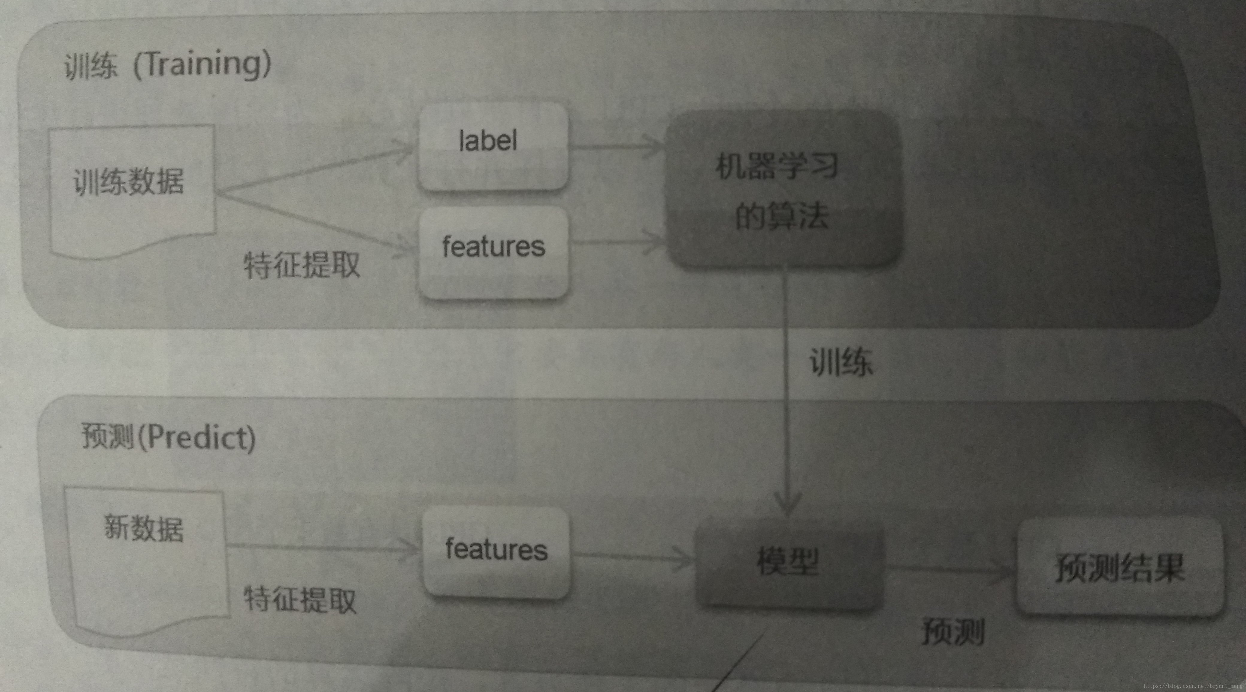
A.1 人工智能、机器学习与深度学习简介

增强式学习，借助定义 Actions、States、Rewards 的方式不断训练机器循序渐进，学会执行某项任务的算法。常用算法有Q-Learning、TD（Temporal Difference）、Sarsa

总结的比较好的一个机器学习框架

A.2 深度学习原理

主要从神经传导原理导入，以 Multilayer Perceptron (MLP) 为例

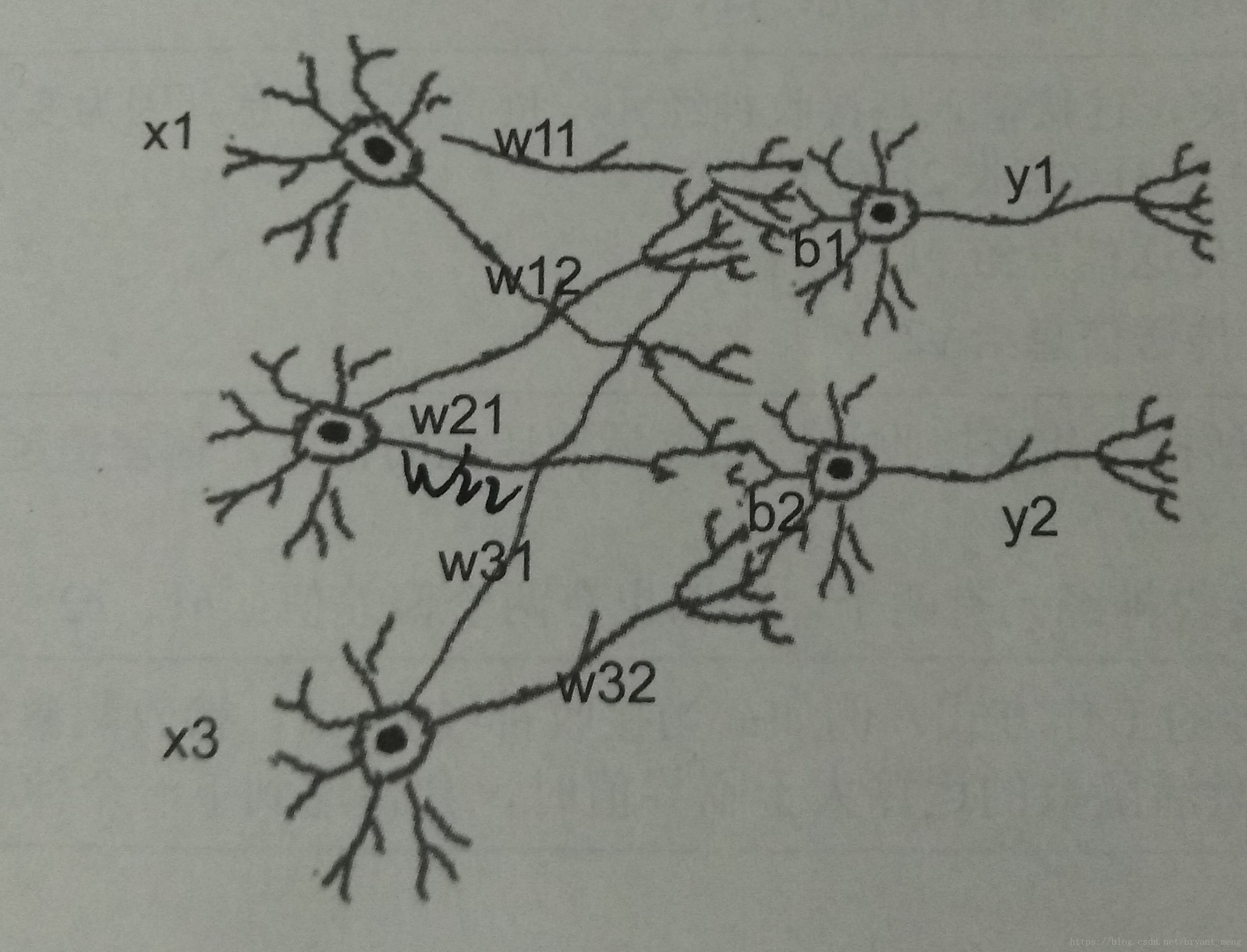
A.2.1 神经传导原理

是我看过的比较销魂的神经网络模型

$\left [y1 \ y2 \right ]= activation\left ( \left [x1 \ x2 \ x3 \right ]\times \begin{bmatrix} w11 & w12\\ w21 & w22\\ w31 & w32 \end{bmatrix} \right )+\left [b1 \ b2 \right ]$
1×2 = 1×3 × 3×2 + 1×2

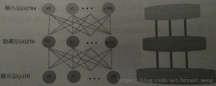
A.2.2 MLP

MNIST
train时，梯度更新，mini-batch，每次读取一批数据进行反向传播算法训练（多样本求均值）

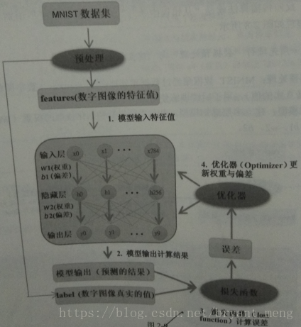
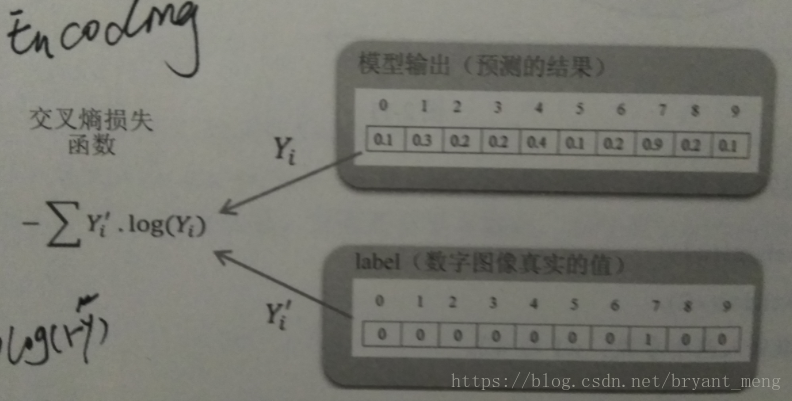
损失函数
one-hot encoding

梯度更新过程

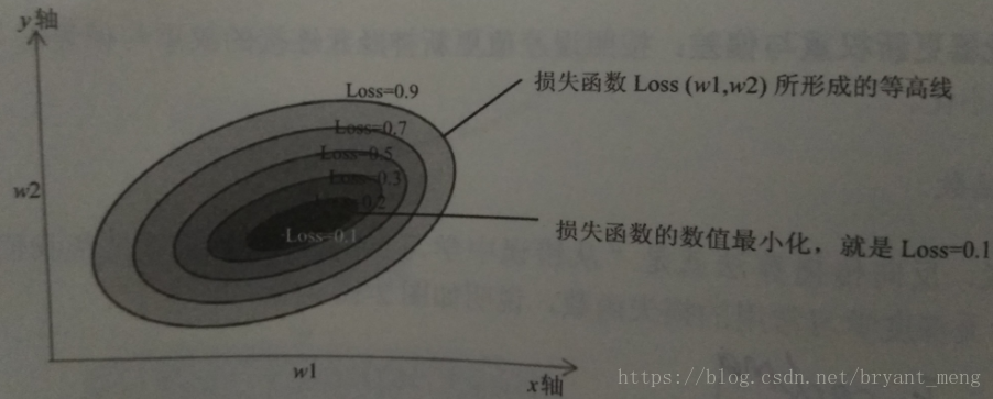
一个样本，算一次梯度，就有一个新的w1和w2。mini-batch，多个样本，多个w1和w2求均值。

A.3 TensorFlow 与 Keras 介绍

TensorFlow：低级深度学习链接库，Brain Team 开发，15年11月公开源码
Keras：高级深度学习链接库

A.3.1 TensorFlow 架构图

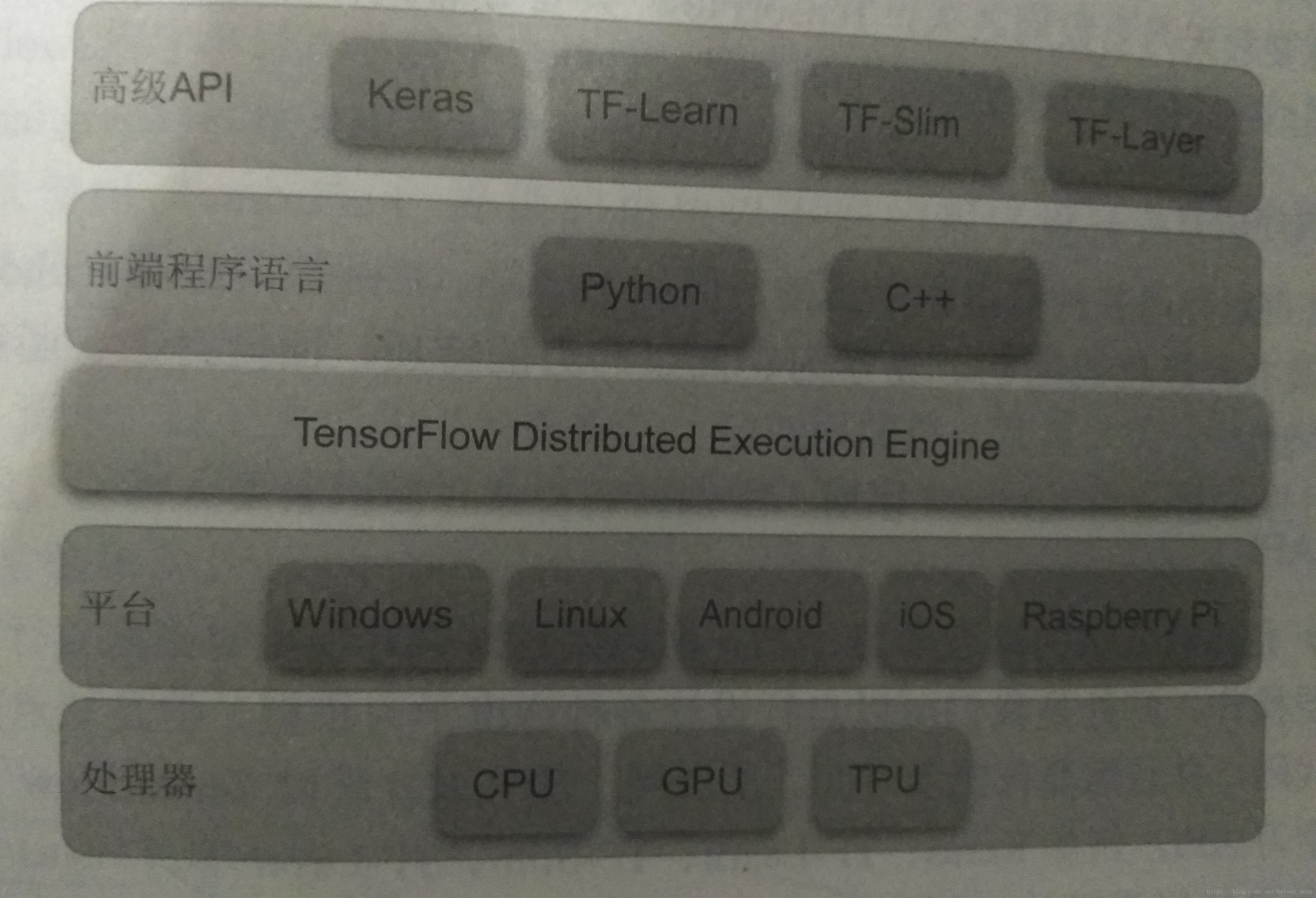
可以跨平台使用，Raspberry Pi树莓派
具备分布式计算能力
前端语言，对 python 支持最好
高级 API，Keras、TF-Learn、TF-Slim、TF-Layer

A.3.2 TensorFlow 简介

1）Tensor（张量）
零维的 Tensor 是标量，1维的是向量，2维以上的是矩阵

2）Flow（数据流）
去陌生的城市，不会当地的语言，最好的方式，画一张图告诉司机你的目的地

computational graph
Node：代表运算（圆圈）
edge：张量的数据流
这里写图片描述

A.3.3 TensorFlow 程序设计模式

核心是computational graph
分为：建立 computational graph 和建立 Session 执行 computational graph

Session（会话）的作用是在客户端和执行设备之间建立连接。有了这个连接，就可以将computational graph在各个不同的设备中执行，后续任何与设备之间的数据传输都必须通过Session来进行，并且最后获得执行后的结果。

tf.Variable（） 构造函数需要变量的初始值，它可以是任何类型和形状的Tensor（张量）。初始值定义变量的类型和形状。施工后，变量的类型和形状是固定的。该值可以使用其中一种赋值方式进行更改。

placeholder, 译为占位符，官方说法:”TensorFlow provides a placeholder operation that must be fed with data on execution.” 即必须在执行时feed值。
placeholder 实例通常用来为算法的实际输入值作占位符。例如，在MNIST例子中，定义输入和输出：

x = tf.placeholder(tf.float32, [None, 784])
#表示成员类型float32， [None, 784]是tensor的shape， None表示第一维是任意数量，784表示第二维是784维
y_ = tf.placeholder(tf.float32, [None, 10])

举个 $y = s i g m o d (W X + b)$ 的例子

import tensorflow as tf
import numpy as np
W =tf.Variable(tf.random_normal([3,2]),name='w') #random_normal,从正态分布中输出随机值。
b =tf.Variable(tf.random_normal([3,2]),name='b')
X = tf.placeholder("float",[None,3],name='X')# placeholder,实例通常用来为算法的实际输入值作占位符
y = tf.nn.sigmoid(tf.matmul(X,W)+b,'y') #激活函数

with tf.Session() as sess:
    init = tf.global_variables_initializer()
    sess.run(init)
    X_array = np.array([[0.4,0.2,0.4],
                      [0.3,0.4,0.5],
                      [0.3,-0.4,0.5]])
    (_b,_W,_X,_y) = sess.run((b,W,X,y),feed_dict={X:X_array})

A.3.4 Keras 介绍

Keras是一个model-level的深度学习链接库，Keras必须配合backend engine 后端引擎（Theano、TensorFlow）进行计算（底层的Tensor计算）。

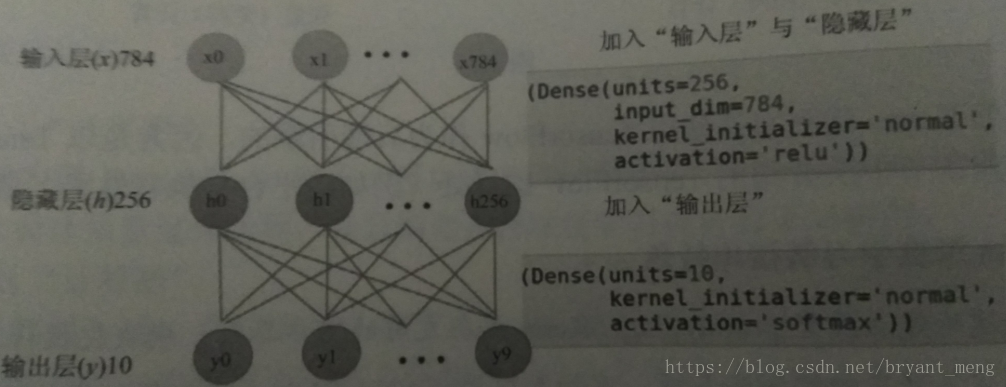
A.3.5 Keras 程序设计模式

蛋糕架+加蛋糕

1）蛋糕架

model = Sequential()

2）加蛋糕

add input and hidden layer in the model
add output layer in the model

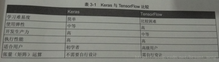
A.3.6 Keras 与 TensorFlow 比较

A.4 在Windows / Linux Ubuntu 中安装TensorFlow 与 Keras

bryant_meng

关注

1
点赞
踩
2

收藏

觉得还不错? 一键收藏
1
评论
《Keras | 莫烦》learning notes

学习资源：Keras 教程系列 | 莫烦 Python参考：《TensorFlow+Keras》Learning notes《Tensorflow | 莫烦》learning notes文章目录1 Why Keras？1.1 Keras 的安装1.2 Backend 的切换2 Classification2.1 MLP for MNIST Classification2.2 ......
复制链接

扫一扫