


本文内容来自学习麻省理工学院公开课:单变量微积分-极限和连续-网易公开课
和麻省理工学院公开课:单变量微积分习题课-分段函数的光滑化-网易公开课
开发环境准备:CSDN
目录
a、 存在, 在x0点的左极限和右极限都存在,同时x0点的左极限等于x0点的右极限
a、跳跃间断,左右两个极限都存在但并不相等,例如上面图显的函数
2、求函数可微的条件(参考下图绿色线,可以发现两部分函数连接处曲线光滑、平顺)
一、极限
1、 抛出公式:
2、求极限的方法:
from sympy import *
x = symbols('x')
expr = x + 1
limit_expr = limit(expr, x, 0)
limit_expr
3、给函数出个图:
import matplotlib.pyplot as plt
import numpy as np
from sympy import *

fig = plt.figure()
ax = fig.add_subplot(1, 1, 1)
ax.spines['left'].set_position('zero')
ax.spines['bottom'].set_position('zero')
ax.spines['right'].set_color('none')
ax.spines['top'].set_color('none')
ax.xaxis.set_ticks_position('bottom')
ax.yaxis.set_ticks_position('left')

x = np.linspace(0,np.pi,50)
y = x + 1
plt.plot(x,y, 'c', label=' fx = x + 1, x >= 0 ')

x = symbols('x')
expr = x + 1
limit_expr = limit(expr, x, 0)
plt.scatter(0, limit_expr, c='r')

x = np.linspace(0,0-np.pi,50)
y = -x + 2
plt.plot(x,y, 'r', label=' fx = -x + 2, x < 0 ')

x = symbols('x')
expr = -x + 2
limit_expr = limit(expr, x, 0)
plt.plot(0,limit_expr,lw=0, marker='o', fillstyle='none')

plt.legend(loc='upper right')

plt.show()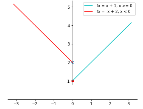
得出的结论是:
二、连续函数和不连续函数
1、函数在点x0连续的条件是:
a、 存在, 在x0点的左极限和右极限都存在,同时x0点的左极限等于x0点的右极限
b、fx在x0点有定义
c、 ( 需要注意的是当计算, 要避免直接计算
  )
)
2、不连续函数
a、跳跃间断,左右两个极限都存在但并不相等,例如上面图显的函数
b、可去间断函数,左右两个极限都存在并相等,例如
fx = x / sin(x)
fx = 1- cos(x) / x
import numpy as np
fig = plt.figure()
ax = fig.add_subplot(1, 1, 1)
ax.spines['left'].set_position('zero')
ax.spines['bottom'].set_position('zero')
ax.spines['right'].set_color('none')
ax.spines['top'].set_color('none')
ax.xaxis.set_ticks_position('bottom')
ax.yaxis.set_ticks_position('left')


# plot the functions x / sin(x)
x = np.linspace(-0.1,-2.5,100)
y = x / np.sin(x)
plt.plot(x,y, 'c', label='y= x / sin(x)')

x = np.linspace(0.1,2.5,100)
y = x / np.sin(x)
plt.plot(x,y, 'c')

x,y = symbols('x y')
expr = x/y
z = expr.subs(y,sin(x)).subs(x,0.1)
z1 = expr.subs(y,sin(x)).subs(x,0)
plt.plot(0,z,lw=0, marker='o', fillstyle='none',label=format(z1), color = 'b')

# plot the functions 1-cos(x)/x
x = np.linspace(-0.1,-2.5,100)
y = (1 - np.cos(x)) / x
plt.plot(x,y, 'r', label='y= (1 - cos(x))/x')

x = np.linspace(0.1,2.5,100)
y = (1 - np.cos(x)) / x
plt.plot(x,y, 'r')

x,y = symbols('x y')
expr = y/x
z = expr.subs(y,1 - cos(x)).subs(x,0.1)
z1 = expr.subs(y, 1- cos(x)).subs(x,0)
plt.plot(0,z,lw=0, marker='o', fillstyle='none', color='b')
plt.legend(loc='upper left')
# show the plot
plt.show()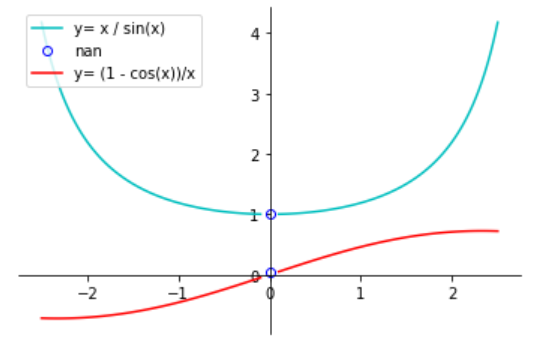
c、无穷间断
,
import numpy as np
import matplotlib.pyplot as plt
fig = plt.figure()
ax = fig.add_subplot(1, 1, 1)
ax.spines['left'].set_position('zero')
ax.spines['bottom'].set_position('zero')
ax.spines['right'].set_color('none')
ax.spines['top'].set_color('none')
ax.xaxis.set_ticks_position('bottom')
ax.yaxis.set_ticks_position('left')
x = np.linspace(-np.pi,-0.1,50)
y = 1 / x
plt.plot(x,y, 'c', label=' fx = 1/x ')
x = np.linspace(0.1,np.pi,50)
y = 1 / x
plt.plot(x,y, 'c')
plt.legend(loc='upper right')
plt.show()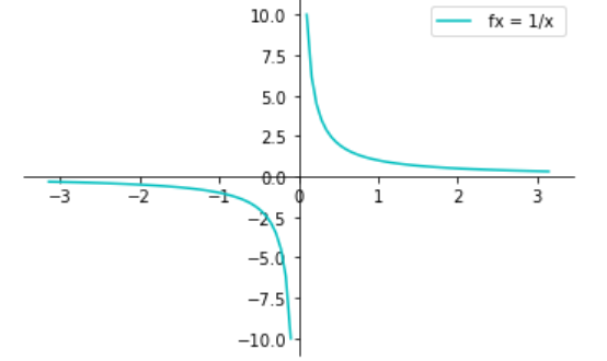
这个函数的导数:
from sympy import *
x = Symbol('x')
f = 1/x
derivative_f = f.diff(x)
derivative_f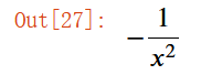
导数的图像:
import numpy as np
import matplotlib.pyplot as plt
fig = plt.figure()
ax = fig.add_subplot(1, 1, 1)
ax.spines['left'].set_position('zero')
ax.spines['bottom'].set_position('zero')
ax.spines['right'].set_color('none')
ax.spines['top'].set_color('none')
ax.xaxis.set_ticks_position('bottom')
ax.yaxis.set_ticks_position('left')
x = np.linspace(-1,-0.1,50)
y = -1 / (x*x)
plt.plot(x,y, 'c', label=' fx = 1/x**2 ')
x = np.linspace(0.1,1,50)
y = -1 / (x*x)
plt.plot(x,y, 'c')
plt.legend(loc='center right')
plt.show()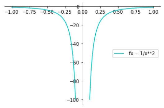
d、其他(丑陋)间断
fx = sin(1/x) 当x趋近于零时,函数值上下反复震荡,但并没有在0点的左极限或右极限
import numpy as np
import sympy
import matplotlib.pyplot as plt
fig = plt.figure()
ax = fig.add_subplot(1, 1, 1)
ax.spines['left'].set_position('zero')
ax.spines['bottom'].set_position('zero')
ax.spines['right'].set_color('none')
ax.spines['top'].set_color('none')
ax.xaxis.set_ticks_position('bottom')
ax.yaxis.set_ticks_position('left')
x = np.linspace(-1,-0.01,50)
y = np.sin(1/x)
plt.plot(x,y, 'c', label=' fx = 1/x**2 ')
x = np.linspace(0.01,1,50)
y = np.sin(1/x)
plt.plot(x,y, 'c')
plt.legend(loc='center right')
plt.show()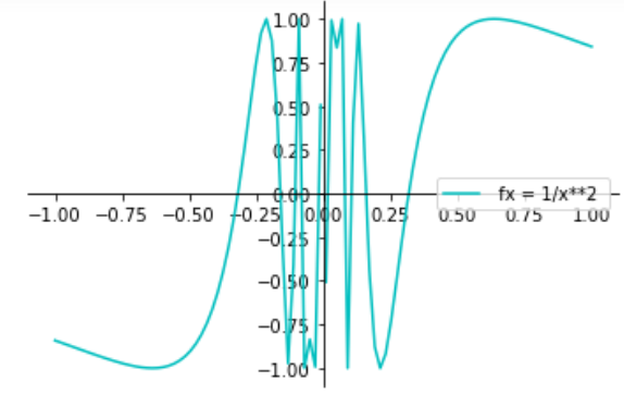
三、定理
当函数f(x)在x0处可导,则这个函数在x0处连续
证明:
当函数在x0处连续的意思就是f(x)在x0处两端的极限有值并几乎等于函数在x0处的值
解:
当x趋近于x0时,
所以有式子 ,而当x趋近于x0时
四、习题
有下列方程组:
问a、b怎样取值可以让函数连续,又怎样取值让函数可微。
1、求连续条件
由 得到函数在x=1时, f(x) = 2, 所以想让f(x)连续,f(x) = ax+b需满足同样得条件。
由 ax+b = 2 , 可以得到多组解, 如 a = 0, b =2; a=1 , b=1; a=2, b=0 等等
2、求函数可微的条件(参考下图绿色线,可以发现两部分函数连接处曲线光滑、平顺)
当函数可微,说明函数导数在x=1的左极限和右极限相等
又因为函数在(1,2)处连续,所以有 2 + b = 0; b=-2
import numpy as np
from sympy import *
import matplotlib.pyplot as plt
fig = plt.figure()
ax = fig.add_subplot(1, 1, 1)
ax.spines['left'].set_position('zero')
ax.spines['bottom'].set_position('zero')
ax.spines['right'].set_color('none')
ax.spines['top'].set_color('none')
ax.xaxis.set_ticks_position('bottom')
ax.yaxis.set_ticks_position('left')
x = np.linspace(1,3,50)
y = x**2 + 1
plt.plot(x,y, 'c', label=' fx = x^2+1 x>1 ')

def MakeXY(valA,valB):
    a,b,x = symbols('a b x')
    expr = a*x+b

    xarr = np.linspace(-3,1,50)
    yarr = []
    for xval in xarr:
        yexpr = expr.subs(x,xval).subs(a,valA).subs(b,valB)
        yarr.append(yexpr)
    y_nparr = np.array(yarr)
    return xarr, y_nparr

def PlotContinueFunc2(plt):
    a,b = symbols('a b');
    expr = a + b
    eqy = Eq(expr.subs(a,0), 2)
    solb = solve(eqy)
    x,y = MakeXY(0,solb[0])
    plt.plot(x, y, color='b', label='y = ax+b ,a = 0, b='+format(solb[0]))
    eqy = Eq(expr.subs(a,1), 2)
    solb = solve(eqy)
    x,y = MakeXY(1,solb[0])
    plt.plot(x, y, color='b', label='y = ax+b ,a = 1, b='+format(solb[0]))
    eqy = Eq(expr.subs(a,2), 2)
    solb = solve(eqy)
    x,y = MakeXY(2,solb[0])
    plt.plot(x, y, color='b', label='y = ax+b ,a = 2, b='+format(solb[0]))
    eqy = Eq(expr.subs(a,3), 2)
    solb = solve(eqy)
    x,y = MakeXY(3,solb[0])
    plt.plot(x, y, color='b', label='y = ax+b ,a = 3, b='+format(solb[0]))


PlotContinueFunc2(plt)
plt.legend(loc='upper right')
plt.show()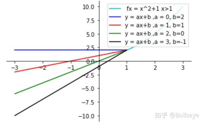


 3296
3296


 被折叠的 条评论
为什么被折叠?
被折叠的 条评论
为什么被折叠?
 到【灌水乐园】发言


