DCGAN论文笔记+源码解析

论文地址：UNSUPERVISED REPRESENTATION LEARNING WITH DEEP CONVOLUTIONAL GENERATIVE ADVERSARIAL NETWORKS

源码地址：DCGAN in TensorFlow

DCGAN，Deep Convolutional Generative Adversarial Networks是生成对抗网络（Generative Adversarial Networks）的一种延伸，将卷积网络引入到生成式模型当中来做无监督的训练，利用卷积网络强大的特征提取能力来提高生成网络的学习效果。

DCGAN有以下特点：

1.在判别器模型中使用strided convolutions来替代空间池化（pooling），而在生成器模型中使用fractional strided convolutions，即deconv，反卷积层。

2.除了生成器模型的输出层和判别器模型的输入层，在网络其它层上都使用了Batch Normalization，使用BN可以稳定学习，有助于处理初始化不良导致的训练问题。

3.去除了全连接层，而直接使用卷积层连接生成器和判别器的输入层以及输出层。

4.在生成器的输出层使用Tanh激活函数，而在其它层使用ReLU；在判别器上使用leaky ReLU。

原论文中只给出了在LSUN实验上的生成器模型的结构图如下：

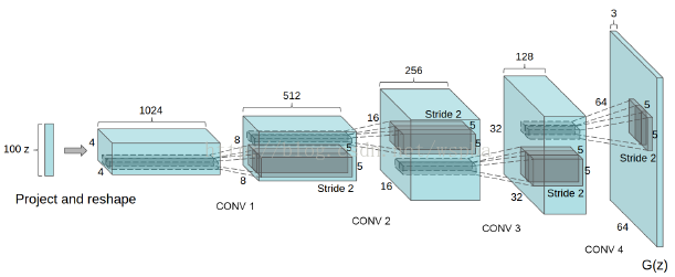
但是对于实验细节以及方法的介绍并不是很详细，于是便从源码入手来理解DCGAN的工作原理。

先看main.py：

with tf.Session(config=run_config) as sess:
  if FLAGS.dataset == 'mnist':
    dcgan = DCGAN(
        sess,
        input_width=FLAGS.input_width,
        input_height=FLAGS.input_height,
        output_width=FLAGS.output_width,
        output_height=FLAGS.output_height,
        batch_size=FLAGS.batch_size,
        y_dim=10,
        c_dim=1,
        dataset_name=FLAGS.dataset,
        input_fname_pattern=FLAGS.input_fname_pattern,
        is_crop=FLAGS.is_crop,
        checkpoint_dir=FLAGS.checkpoint_dir,
        sample_dir=FLAGS.sample_dir)

因为我们使用DCGAN来生成MNIST数字手写体图像，注意这里的y_dim=10，表示0到9这10个类别，c_dim=1，表示灰度图像。

再看model.py：

def discriminator(self, image, y=None, reuse=False):
  with tf.variable_scope("discriminator") as scope:
    if reuse:
      scope.reuse_variables()

    yb = tf.reshape(y, [self.batch_size, 1, 1, self.y_dim])
    x = conv_cond_concat(image, yb)

    h0 = lrelu(conv2d(x, self.c_dim + self.y_dim, name='d_h0_conv'))
    h0 = conv_cond_concat(h0, yb)

    h1 = lrelu(self.d_bn1(conv2d(h0, self.df_dim + self.y_dim, name='d_h1_conv')))
    h1 = tf.reshape(h1, [self.batch_size, -1])      
    h1 = tf.concat_v2([h1, y], 1)
       
    h2 = lrelu(self.d_bn2(linear(h1, self.dfc_dim, 'd_h2_lin')))
    h2 = tf.concat_v2([h2, y], 1)

    h3 = linear(h2, 1, 'd_h3_lin')
        
    return tf.nn.sigmoid(h3), h3

这里batch_size=64，image的维度为[64 28 28 1]，y的维度是[64 10]，yb的维度[64 1 1 10]，x将image和yb连接起来，这相当于是使用了Conditional GAN，为图像提供标签作为条件信息，于是x的维度是[64 28 28 11]，将x输入到卷积层conv2d，conv2d的代码如下：

def conv2d(input_, output_dim, 
       k_h=5, k_w=5, d_h=2, d_w=2, stddev=0.02,
       name="conv2d"):
  with tf.variable_scope(name):
    w = tf.get_variable('w', [k_h, k_w, input_.get_shape()[-1], output_dim],
              initializer=tf.truncated_normal_initializer(stddev=stddev))
    conv = tf.nn.conv2d(input_, w, strides=[1, d_h, d_w, 1], padding='SAME')

    biases = tf.get_variable('biases', [output_dim], initializer=tf.constant_initializer(0.0))
    conv = tf.reshape(tf.nn.bias_add(conv, biases), conv.get_shape())

    return conv

卷积核的大小为5*5，stride为[1 2 2 1]，通过2的卷积步长可以替代pooling进行降维，padding=‘SAME’，则卷积的输出维度为[64 14 14 11]。然后使用batch normalization及leaky ReLU的激活层，输出与yb再进行concat，得到h0，维度为[64 14 14 21]。同理，h1的维度为[64  7*7*74+10]，h2的维度为[64 1024+10]，然后连接一个线性输出，得到h3，维度为[64 1]，由于我们希望判别器的输出代表概率，所以最终使用一个sigmoid的激活。

def generator(self, z, y=None):
  with tf.variable_scope("generator") as scope:
      
    s_h, s_w = self.output_height, self.output_width
    s_h2, s_h4 = int(s_h/2), int(s_h/4)
    s_w2, s_w4 = int(s_w/2), int(s_w/4)

    # yb = tf.expand_dims(tf.expand_dims(y, 1),2)
    yb = tf.reshape(y, [self.batch_size, 1, 1, self.y_dim])
    z = tf.concat_v2([z, y], 1)

    h0 = tf.nn.relu(
        self.g_bn0(linear(z, self.gfc_dim, 'g_h0_lin')))
    h0 = tf.concat_v2([h0, y], 1)

    h1 = tf.nn.relu(self.g_bn1(
        linear(h0, self.gf_dim*2*s_h4*s_w4, 'g_h1_lin')))
    h1 = tf.reshape(h1, [self.batch_size, s_h4, s_w4, self.gf_dim * 2])

    h1 = conv_cond_concat(h1, yb)

    h2 = tf.nn.relu(self.g_bn2(deconv2d(h1,
        [self.batch_size, s_h2, s_w2, self.gf_dim * 2], name='g_h2')))
    h2 = conv_cond_concat(h2, yb)

    return tf.nn.sigmoid(
        deconv2d(h2, [self.batch_size, s_h, s_w, self.c_dim], name='g_h3'))

output_height和output_width为28，因此s_h和s_w为28，s_h2和s_w2为14，s_h4和s_w4为7。在这里z为平均分布的随机分布数，维度为[64 100]，y的维度为[64 10]，yb的维度是[64 1 1 10]，z与y进行一个concat得到[64 110]的tensor，输入到一个线性层，输出维度是[64 1024]，再经过batch normalization以及ReLU激活，并与y进行concat，输出h0的维度是[64 1034]，同样的再经过一个线性层输出维度为[64 128*7*7]，再进行reshape并与yb进行concat，得到h1，维度为[64 7 7 138]，然后输入到一个deconv2d，做一个反卷积，也就是文中说的fractional strided convolutions，再经过batch normalization以及ReLU激活，并与yb进行concat，输出h2的维度是[64 14 14 138]，最后再输入到deconv2d层以及sigmoid激活，得到生成器的输出，维度为[64 28 28 1]。

生成器以及判别器的输出：

self.G = self.generator(self.z, self.y)
self.D, self.D_logits = \
    self.discriminator(inputs, self.y, reuse=False)

self.D_, self.D_logits_ = \
    self.discriminator(self.G, self.y, reuse=True)

其中D表示真实数据的判别器输出，D_表示生成数据的判别器输出。

再看损失函数：

self.d_loss_real = tf.reduce_mean(
  tf.nn.sigmoid_cross_entropy_with_logits(
    logits=self.D_logits, targets=tf.ones_like(self.D)))
self.d_loss_fake = tf.reduce_mean(
  tf.nn.sigmoid_cross_entropy_with_logits(
    logits=self.D_logits_, targets=tf.zeros_like(self.D_)))
self.g_loss = tf.reduce_mean(
  tf.nn.sigmoid_cross_entropy_with_logits(
    logits=self.D_logits_, targets=tf.ones_like(self.D_)))

即对于真实数据，判别器的损失函数d_loss_real为判别器输出与1的交叉熵，而对于生成数据，判别器的损失函数d_loss_fake为输出与0的交叉熵，因此判别器的损失函数d_loss=d_loss_real+d_loss_fake；生成器的损失函数是g_loss判别器对于生成数据的输出与1的交叉熵。
优化器：

d_optim = tf.train.AdamOptimizer(config.learning_rate, beta1=config.beta1) \
          .minimize(self.d_loss, var_list=self.d_vars)
g_optim = tf.train.AdamOptimizer(config.learning_rate, beta1=config.beta1) \
          .minimize(self.g_loss, var_list=self.g_vars)

训练阶段：

for epoch in xrange(config.epoch):
  batch_idxs = min(len(data_X), config.train_size) // config.batch_size
      
  for idx in xrange(0, batch_idxs):
        
    batch_images = data_X[idx*config.batch_size:(idx+1)*config.batch_size]
    batch_labels = data_y[idx*config.batch_size:(idx+1)*config.batch_size]
 
    batch_images = np.array(batch).astype(np.float32)[:, :, :, None]
 
    batch_z = np.random.uniform(-1, 1, [config.batch_size, self.z_dim]) \
          .astype(np.float32)

    # Update D network
    _, summary_str = self.sess.run([d_optim, self.d_sum],
      feed_dict={ 
        self.inputs: batch_images,
        self.z: batch_z,
        self.y:batch_labels,
      })
    self.writer.add_summary(summary_str, counter)

    # Update G network
    _, summary_str = self.sess.run([g_optim, self.g_sum],
      feed_dict={
        self.z: batch_z, 
        self.y:batch_labels,
      })
    self.writer.add_summary(summary_str, counter)

    # Run g_optim twice to make sure that d_loss does not go to zero (different from paper)
    _, summary_str = self.sess.run([g_optim, self.g_sum],
      feed_dict={ self.z: batch_z, self.y:batch_labels })
    self.writer.add_summary(summary_str, counter)
        
    errD_fake = self.d_loss_fake.eval({
        self.z: batch_z, 
        self.y:batch_labels
    })
    errD_real = self.d_loss_real.eval({
        self.inputs: batch_images,
        self.y:batch_labels
    })
    errG = self.g_loss.eval({
        self.z: batch_z,
        self.y: batch_labels
    })
     
    counter += 1

与论文中不同的是，这里在一个batch中，更新两次生成器，更新一次判别器。

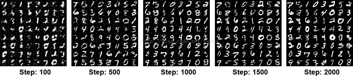
实验结果：

由于自己的笔记本配置有限，仅使用CPU来运行速度较慢，因此epoch仅设置为2，对于MNIST手写数字数据集的生成情况如下

注1：发现代码中以mnist为训练集的网络和以无标签数据集（以下简称unlabeled_dataset）为训练集的网络不同，结构有别。以下笔记主要针对前者(Generator=3个ReLU+1个Sigmoid，Discriminator=3个LeakyReLU+1个Sigmoid)。

注2：事实上，以unlabeled_dataset为训练集的网络也同原网页中所画的Generator有一些不同（事实上，区别是每个conv层的filter个数被减半了。原因可能为了减少网络参数利于测试者训练？）。除此以外，结构相同。Discriminator的结构与Generator的结构正好对称。

 

原代码中对于有label的数据集，Generator和Discriminator的网络结构均只有两个卷积层。

预备：batch_size=64, mnist图片大小28*28*c_dim，其中c_dim=1为颜色维数，类别数10；随机输入维数z_dim=100

Generator 部分

step1（获得输入z）：服从均匀分布的输入样本z（shape=64,100）与具有one-hot形式的标签y (shape=64,10)级联，整体作为Generator的输入z (shape=64,110)

step2（获得第一个非线性层的输出h0）： 通过线性变换将z变换为维数为gfc_dim=1024的数据，对其块归一化之后进行非线性ReLU变换，得到h0 （shape=64,1024）；将h0与y级联，整体作为下一层的输入h0 （shape=64,1034）

step3（获得第二个非线性层的输出h1）：通过线性变换将h0变换为维数为128*7*7=6272的数据，对其块归一化之后进行非线性ReLU变换，得到h1 （shape=64,6272）；将h1进行reshape操作得到h1（shape=64,7,7,128）；将h1与yb（yb为y的reshape形式，即最后一维为label维，yb的shape=64,1,1,10）级联，整体作为下一层的输入h1 （shape=64,7,7,139）

step4（获得第三个非线性层的输出h2）：通过deconv2d操作，用128个filter，将h1变换为维数为64*14*14*128的数据，对其块归一化之后进行非线性ReLU变换，得到h2 （shape=64,14,14,128）；将h2与yb级联，整体作为下一层的输入h2 （shape=64,14,14,139）

step5（获得最终的生成图像generated_image）：通过deconv2d操作，用c_dim个filter，将h1变换为维数为64*28*28*1的数据，不做块归一化，进行非线性Sigmoid变换，得到generated_image（shape=64,28,28,1）

Discriminator 部分

step1（获得输入x）：真实/生成图像image（shape=64,28,28,1）和yb（shape=64,1,1,10）级联，整体作为Discriminator的输入x（shape=64,28,28,11）

step2（获得第一个卷积层的输出h0）：用c_dim+y_dim=1+10=11个大小为5*5*11的filter对输入x进行二维卷积操作，随后进行非线性LeakyReLU变换，得到h0 （shape=64,14,14,11）；将h0与标签yb级联，整体作为下一层的输入h0（shape=64,14,14,21）

step3（获得第二个卷积层的输出h1）：用df_dim+y_dim=64+10=74个大小为5*5*21的filter对h0进行二维卷积操作，块归一化(这层有)之后进行非线性LeakReLU变换，得到h1（shape=64,7,7,74）；对h1进行reshape拉成每个样本对应一维数据，并与标签y (shape=64,10)级联，整体作为下一层的输入h1（shape=64,7*7*74+10=64,3636）

step4（获得第三个卷积层的输出h2）：对h1进行线性变换，输出维数为dfc_dim=1024的数据，块归一化(这层有)操作之后进行非线性LeakyReLU变换，得到h2 （shape=64,1024）；将h2与y进行级联，整体作为下一层的输入h2（shape=64,1034）

step5（获得最终输出h3）：对h2进行线性变换，输出维数为1（用来判断真假）的数据，非线性Sigmoid变换之后得到最终输出h3 (shape=64,1)  (注：实际代码中将线性变换之后的结果也进行了输出，用以计算loss)

Loss部分

真实图像和生成图像这两种图像都需要输入Discriminator得到对应的loss，整体作为Discriminator的loss；

而Generator的loss只包含有关生成图像部分；

用Adam训练，每训练两次Generator，才对Discriminator进行一次训练，防止Discriminator的loss的导数为0(无法更新)。

 

好吧，这样看着代码写出来的步骤简直太吃藕了，咱来用一下TensorBoard的功能，Generator和Discriminator的结构大概如下：