Splatter Image: Ultra-Fast Single-View 3D Reconstruction

Splatter Image: Ultra-Fast Single-View 3D Reconstruction
飞溅图像：超快速单视图3D重建

Stanislaw Szymanowicz  Christian Rupprecht  Andrea Vedaldi
克里斯蒂安·鲁普雷希特·安德烈·韦达尔迪
Visual Geometry Group — University of Oxford {stan,chrisr,vedaldi}@robots.ox.ac.uk
视觉几何组-牛津大学{stan，chrisr，vedaldi}@robots.ox.ac.uk

Abstract 摘要     [2312.13150] Splatter Image: Ultra-Fast Single-View 3D Reconstruction

We introduce the Splatter Image 11Website: szymanowiczs.github.io/splatter-image
网址：szymanowiczs.github.io/splatter-image
我们介绍飞溅图像 1, an ultra-fast approach for monocular 3D object reconstruction which operates at 38 FPS. Splatter Image is based on Gaussian Splatting, which has recently brought real-time rendering, fast training, and excellent scaling to multi-view reconstruction. For the first time, we apply Gaussian Splatting in a monocular reconstruction setting. Our approach is learning-based, and, at test time, reconstruction only requires the feed-forward evaluation of a neural network. The main innovation of Splatter Image is the surprisingly straightforward design: it uses a 2D image-to-image network to map the input image to one 3D Gaussian per pixel. The resulting Gaussians thus have the form of an image, the Splatter Image. We further extend the method to incorporate more than one image as input, which we do by adding cross-view attention. Owning to the speed of the renderer (588 FPS), we can use a single GPU for training while generating entire images at each iteration in order to optimize perceptual metrics like LPIPS. On standard benchmarks, we demonstrate not only fast reconstruction but also better results than recent and much more expensive baselines in terms of PSNR, LPIPS, and other metrics.
，一种用于单目3D物体重建的超快速方法，其操作速度为38 FPS。Splatter Image是基于Gaussian Splatting的，它最近为多视图重建带来了实时渲染，快速训练和出色的缩放。这是我们第一次在单目重建环境中应用高斯溅射。我们的方法是基于学习的，并且在测试时，重建只需要神经网络的前馈评估。Splatter Image的主要创新是令人惊讶的简单设计：它使用2D图像到图像网络将输入图像映射到每个像素的3D高斯。由此产生的高斯因此具有图像的形式，即飞溅图像。我们进一步扩展的方法，将一个以上的图像作为输入，我们通过添加跨视图的注意。 由于渲染器的速度（588 FPS），我们可以使用单个GPU进行训练，同时在每次迭代时生成整个图像，以优化LPIPS等感知指标。在标准基准测试中，我们不仅展示了快速重建，而且在PSNR，LPIPS和其他指标方面比最近更昂贵的基线有更好的结果。

Figure 1: The Splatter Image is an ultra-fast method for single- and few-view 3D reconstruction. It works by applying an image-to-image neural network to the input view and obtain, as output, another image that holds the parameters of one coloured 3D Gaussian per pixel. The resulting Gaussian mixture can be rendered very quickly into an arbitrary view of the object by using Gaussian Splatting.
图1：Splatter Image是一种用于单视图和少视图3D重建的超快速方法。它的工作原理是将图像到图像神经网络应用于输入视图，并获得另一个图像作为输出，该图像包含每个像素的一个彩色3D高斯参数。通过使用高斯溅射，可以非常快速地将所得到的高斯混合渲染成对象的任意视图。

1Introduction 1介绍

Single-view 3D reconstruction poses a fundamental challenge in computer vision. In this paper, we contribute Splatter Image, a method that achieves ultra-fast single-view reconstruction of the 3D shape and appearance of objects. This method uses Gaussian Splatting [14] as the underlying 3D representation, taking advantage of its rendering quality and speed. It works by predicting a 3D Gaussian for each of the input image pixels, using an image-to-image neural network. Remarkably, the 3D Gaussians in the resulting ‘Splatter Image’ provide 360∘ reconstructions (Fig. 1) of quality matching or outperforming much slower methods.
单视图三维重建是计算机视觉中的一个基本挑战。在本文中，我们贡献飞溅图像，一种方法，实现超快速的单视图重建的3D形状和外观的对象。该方法使用高斯飞溅[14]作为底层3D表示，利用其渲染质量和速度。它的工作原理是使用图像到图像神经网络为每个输入图像像素预测3D高斯。值得注意的是，结果“飞溅图像”中的3D高斯提供了360 ∘ 重建（图1）的质量匹配或优于慢得多的方法。

The key challenge in using 3D Gaussians for monocular reconstruction is to design a network that takes an image of an object as input and produces as output a corresponding Gaussian mixture that represents all sides of it. We note that, while a Gaussian mixture is a set, i.e., an unordered collection, it can still be stored in an ordered data structure. Splatter Image takes advantage of this fact by using a 2D image as a container for the 3D Gaussians, so that each pixel contains in turn the parameters of one Gaussian, including its opacity, shape, and colour.
使用3D高斯进行单目重建的关键挑战是设计一个网络，该网络将对象的图像作为输入，并产生表示其所有侧面的相应高斯混合作为输出。我们注意到，虽然高斯混合是一个集合，即，一个无序的集合，它仍然可以存储在一个有序的数据结构中。Splatter Image利用了这一点，使用2D图像作为3D高斯的容器，因此每个像素都包含一个高斯的参数，包括其不透明度，形状和颜色。

The advantage of storing sets of 3D Gaussians in an image is that it reduces the reconstruction problem to learning an image-to-image neural network. In this manner, the reconstructor can be implemented utilizing only efficient 2D operators (e.g., 2D convolution instead of 3D convolution). We use in particular a U-Net [32] as those have demonstrated excellent performance in image generation [31]. In our case, their ability to capture small image details [44] helps to obtain higher-quality reconstructions.
在图像中存储3D高斯集的优点是它将重建问题减少到学习图像到图像神经网络。以这种方式，可以仅利用有效的2D算子（例如，2D卷积而不是3D卷积）。我们特别使用U-Net [32]，因为它们在图像生成[31]方面表现出出色的性能。在我们的案例中，他们捕捉小图像细节的能力[44]有助于获得更高质量的重建。

Since the 3D representation in Splatter Image is a mixture of 3D Gaussians, it enjoys the rendering speed and memory efficiency of Gaussian Splatting, which is advantageous both in inference and training. In particular, rendering stops being a training bottleneck and we can afford to generate complete views of the object to optimize perceptual metrics like LPIPS [45]. Possibly even more remarkably, the efficiency is such that our model can be trained on a single GPU on standard benchmarks of 3D objects, whereas alternative methods typically require distributed training on several GPUs. We also extend Splatter Image to take several views as input. This is achieved by taking the union of the Gaussian mixtures predicted from individual views, after registering them to a common reference. Furthermore, we allow different views to communicate during prediction by injecting lightweight cross-view attention layers in the architecture.
由于Splatter Image中的3D表示是3D高斯的混合，因此它具有高斯Splatting的渲染速度和内存效率，这在推理和训练方面都具有优势。特别是，渲染不再是训练瓶颈，我们可以生成对象的完整视图，以优化LPIPS等感知指标[45]。可能更值得注意的是，效率是这样的，我们的模型可以在3D对象的标准基准上在单个GPU上进行训练，而其他方法通常需要在多个GPU上进行分布式训练。我们还扩展了Splatter Image，以将多个视图作为输入。这是通过将从各个视图预测的高斯混合物的并集（union）在将它们配准到公共参考之后实现的。此外，我们允许不同的视图在预测过程中进行通信，通过在架构中注入轻量级的跨视图注意层。

Empirically, we study several properties of Splatter Image. First, we note that, while the network only sees one side of the object, it can still produce a 360∘ reconstruction of it by using the prior acquired during training. The 360∘ information is coded in the 2D image by allocating different Gaussians in a given 2D neighbourhood to different parts of the 3D object. We also show that many Gaussians are in practice inactivated by setting their opacity to zero, and can thus be culled in post-processing. We further validate Splatter Image by comparing it to alternative, slower reconstructors on standard benchmark datasets like ShapeNet [4] and CO3D [28]. Compared to these slower baselines, Splatter Image is not only competitive in terms of quality, but in fact state-of-the-art in several cases, improving both reconstruction PSNR and LPIPS. We argue that this is because the very efficient design allows training the model more effectively, including using image-level losses like LPIPS.
在实验上，我们研究了飞溅图像的几个性质。首先，我们注意到，虽然网络只能看到物体的一面，但它仍然可以通过使用训练期间获得的先验知识来生成360 ∘ 重建。通过将给定2D邻域中的不同高斯分配给3D对象的不同部分，在2D图像中对360 ∘ 信息进行编码。我们还表明，许多高斯在实践中通过将其不透明度设置为零来灭活，因此可以在后处理中剔除。我们通过将其与标准基准数据集（如ShapeNet [4]和CO3D [28]）上的替代，较慢的重建器进行比较，进一步验证了Splatter Image。与这些较慢的基线相比，Splatter Image不仅在质量方面具有竞争力，而且在某些情况下实际上是最先进的，可以提高重建PSNR和LPIPS。 我们认为这是因为非常高效的设计可以更有效地训练模型，包括使用像LPIPS这样的图像级损失。

To summarise, our contributions are: (1) to port Gaussian Splatting to learning-based monocular reconstruction; (2) to do so with the Splatter Image, a straightforward, efficient and performant 3D reconstruction approach that operates at 38 FPS on a standard GPU; (3) to also extend the method to multi-view reconstruction; (4) and to obtain state-of-the-art reconstruction performance in standard benchmarks in terms of reconstruction quality and speed.
概括起来，我们的贡献是：（1）将高斯溅射移植到基于学习的单目重建中;（2）使用Splatter Image这样做，这是一种简单，高效和高性能的3D重建方法，在标准GPU上以38 FPS运行;（3）还将该方法扩展到多视图重建;（4）并在重建质量和速度方面在标准基准中获得最先进的重建性能。

2Related work 2相关工作

Representations for single-view 3D reconstruction.
用于单视图3D重建的表示。

In recent years, implicit representations like NeRF [24] have dominated learning-based few-view reconstruction. Some works have approached this problem by parameterising the MLP in NeRF using global [12, 29], local [44] or both global and latent codes [16]. However, implicit representations, particularly MLP-based ones, are notoriously slow to render, up to 2s for a single 128×128 image.
近年来，像NeRF [24]这样的隐式表示已经主导了基于学习的少视图重建。一些工作已经通过使用全局[12，29]，局部[44]或全局和潜在代码[16]来参数化NeRF中的MLP来解决这个问题。然而，隐式表示，特别是基于MLP的表示，渲染速度非常慢，单个 128×128 图像的渲染速度高达2s。

Some follow-up works [8, 38] have used faster implicit representations based on voxel grids that encode opacities and colours directly [8, 38] — similar to DVGO [37], they can thus achieve significant speed-ups. However, due to their voxel-based representation, they scale poorly with resolution. They also assume the knowledge of the absolute viewpoint of each object image.
一些后续工作[8，38]使用了更快的隐式表示，基于直接编码不透明度和颜色的体素网格[8，38] -类似于DVGO [37]，因此可以实现显着的速度提升。然而，由于它们基于体素的表示，它们的分辨率很差。它们还假设每个对象图像的绝对视点的知识。

A hybrid implicit-explicit triplane representation [2] has been proposed as a compromise between rendering speed and memory consumption. Triplanes can be predicted by networks in the camera view space, instead of a global reference frame, thus allowing reconstruction in the view-space [7]. While they are not as fast to render as explicit representations, they are fast enough to be effectively used for single-view reconstruction [1, 7].
隐式-显式混合三平面表示[2]已被提出作为渲染速度和内存消耗之间的折衷。三平面可以通过相机视图空间中的网络来预测，而不是全局参考帧，从而允许在视图空间中重建[7]。虽然它们的渲染速度不如显式表示，但它们足够快，可以有效地用于单视图重建[1，7]。

Finally, several works predict multi-view images directly [3, 19, 39, 42]. 3D models can then be obtained with test-time multi-view optimisation. The main disadvantage of image-to-image novel view generators is that they exhibit noticeable flicker and are 3D inconsistencies, thus limiting the quality of obtained reconstructions. In addition, test-time optimisation is an additional overhead, limiting the overall reconstruction speed.
最后，一些作品直接预测多视图图像[3，19，39，42]。然后可以通过测试时多视图优化获得3D模型。图像到图像新视图生成器的主要缺点是它们表现出明显的闪烁并且是3D不一致的，从而限制了所获得的重建的质量。此外，测试时间优化是额外的开销，限制了整体重建速度。

In contrast to these works, our method predicts a mixture of 3D Gaussians in a feed-forward manner. As a result, our method is fast at inference and achieves real-time rendering speeds while achieving state-of-the-art image quality across multiple metrics on the standard single-view reconstruction benchmark ShapeNet-SRN [35].
与这些工作相反，我们的方法以前馈方式预测3D高斯的混合物。因此，我们的方法推理速度快，实现了实时渲染速度，同时在标准单视图重建基准ShapeNet-SRN [35]上实现了多个指标的最新图像质量。

When more than one view is available at the input, one can learn to interpolate between available views in the 3D space to estimate the scene geometry [5, 21], learn a view interpolation function [41] or optimize a 3D representation of a scene using semantic priors [11]. Our method is primarily a single-view reconstruction network, but we do show how Splatter Image can be extended to fuse multiple views. However, we focus our work on object-centric reconstruction rather than on generalising to unseen scenes.
当输入端有多个视图可用时，可以学习在3D空间中的可用视图之间进行插值以估计场景几何结构[5，21]，学习视图插值函数[41]或使用语义先验优化场景的3D表示[11]。我们的方法主要是单视图重建网络，但我们展示了如何扩展Splatter Image以融合多个视图。然而，我们的工作重点是以对象为中心的重建，而不是概括看不见的场景。

3D Reconstruction with Point Clouds.
点云三维重建。

PointOutNet [9] adapted PointNet [27] to take image encoding as input and trained point cloud prediction networks using 3D point cloud supervision. PVD [46] and PC2 [23] extended this approach using Diffusion Models [10] by conditioning the denoising process on partial point clouds and RGB images, respectively. These approaches require ground truth 3D point clouds, limiting their applicability. Other works [17, 30, 43] train networks for Novel Views Synthesis purely from videos and use point clouds as intermediate 3D representations for conditioning 2D inpainting or generation networks. However, these point clouds are assumed to correspond to only visible object points. In contrast, our Gaussians can model any part of the object, and thus afford 360∘ reconstruction.
PointOutNet [9]将PointNet [27]调整为将图像编码作为输入，并使用3D点云监督训练点云预测网络。PVD [46]和PC 2 [23]通过分别在部分点云和RGB图像上调节去噪过程，使用扩散模型[10]扩展了这种方法。这些方法需要地面实况3D点云，限制了它们的适用性。其他作品[17，30，43]纯粹从视频中训练网络进行新颖视图合成，并使用点云作为中间3D表示来调节2D修复或生成网络。然而，这些点云被假定为仅对应于可见对象点。相比之下，我们的高斯模型可以对物体的任何部分进行建模，从而提供360 ∘ 重建。

Point cloud-based representations have also been used for high-quality reconstruction from multi-view images. ADOP [33] used points with a fixed radius and also used 2D inpainting networks for hole-filling. Gaussian Splatting [14] used non-isotropic 3D Gaussians with variable scale, thus removing the need for 2D inpainting networks. While showing high-quality results, Gaussian Splatting requires many images per scene and has not yet been used in a learning-based reconstruction framework as we do here.
基于点云的表示也已用于从多视图图像进行高质量重建。ADOP [33]使用具有固定半径的点，并使用2D修补网络进行孔洞填充。高斯溅射[14]使用具有可变尺度的非各向同性3D高斯，从而消除了对2D修复网络的需求。虽然高斯溅射显示高质量的结果，但每个场景需要许多图像，并且还没有像我们在这里所做的那样用于基于学习的重建框架。

Our method also uses 3D Gaussians as an underlying representation but predicts them from as few as a single image. Moreover, it outputs a full 360∘ 3D reconstruction without using 2D or 3D inpainting networks.
我们的方法还使用3D高斯作为底层表示，但仅从单个图像中预测它们。此外，它输出完整的360 ∘ 3D重建，而不使用2D或3D修复网络。

Probabilistic 3D Reconstruction.
可能的3D重建。

Single-view 3D reconstruction is an ambiguous problem, so several authors argue that it should be tackled as a conditional generative problem. Diffusion Models have been employed for conditional Novel View Synthesis [3, 42, 19, 18]. Due to generating images without underlying geometries, the output images exhibit noticeable flicker. This can be mitigated by simultaneously generating multi-view images [20, 34], or guaranteed by reconstructing a geometry at every step of the denoising process [38, 40]. Other works build and use a 3D [25, 6] or 2D [7, 22] prior which can be used in an image-conditioned auto-decoding framework.
单视图三维重建是一个模糊的问题，所以一些作者认为，它应该作为一个条件生成的问题来解决。扩散模型已被用于有条件的新视图合成[3，42，19，18]。由于生成的图像没有底层几何图形，因此输出图像会出现明显的闪烁。这可以通过同时生成多视图图像[20，34]来缓解，或者通过在去噪过程的每个步骤中重建几何结构来保证[38，40]。其他作品构建并使用3D [25，6]或2D [7，22]先验，可用于图像调节的自动解码框架。

Here, we focus on deterministic reconstruction. However, few-view reconstruction is required to output 3D geometries from feed-forward methods  [20, 34, 38, 40]. Our method is capable of few-view 3D reconstruction, thus it is complimentary to these generative methods and could lead to improvements in generation speed and quality.
在这里，我们专注于确定性重建。然而，需要少视图重建来从前馈方法输出3D几何形状[20，34，38，40]。我们的方法是能够少视图的三维重建，因此它是互补的，这些生成方法，并可能导致生成速度和质量的提高。

3Method 3方法

We provide background information on Gaussian Splatting in Sec. 3.1, and then describe the Splatter Image in Secs. 3.2, 3.3, 3.4, 3.5 and 3.6.
我们提供了关于高斯溅射的背景信息。3.1，然后以秒为单位描述飞溅图像。3.2、3.3、3.4、3.5和3.6。

3.1Overview of Gaussian Splatting
3.1高斯溅射概述

A radiance field [24] is given by the opacity function 𝜎​(𝒙)∈ℝ+ and the colour function 𝑐​(𝒙,𝝂)∈ℝ3, where 𝝂∈𝕊2 is the viewing direction of the 3D point 𝒙∈ℝ3.
辐射场[24]由不透明度函数 𝜎​(𝒙)∈ℝ+ 和颜色函数 𝑐​(𝒙,𝝂)∈ℝ3 给出，其中 𝝂∈𝕊2 是3D点 𝒙∈ℝ3 的观察方向。

The field is rendered onto an image 𝐼​(𝒖) by integrating the colors observed along the ray 𝒙𝜏=𝒙0−𝜏​𝝂, 𝜏∈ℝ+ that passes through pixel 𝒖:
通过对沿着穿过像素 𝒖 的光线 𝒙𝜏=𝒙0−𝜏​𝝂 、 𝜏∈ℝ+ 观察到的颜色进行积分，将场渲染到图像 𝐼​(𝒖) 上：

𝐼​(𝒖)=∫0∞𝑐​(𝒙𝜏,𝝂)​𝜎​(𝒙𝜏)​𝑒−∫0𝜏𝜎​(𝒙𝜇)​𝑑𝜇​𝑑𝜏.

(1)

Gaussian Splatting [48] represents these two functions as a mixture 𝜃 of 𝐺 colored Gaussians
高斯溅射[48]将这两个函数表示为 𝜃 和 𝐺 有色高斯的混合

𝑔𝑖​(𝒙)=exp⁡(−12​(𝒙−𝝁𝑖)⊤​Σ𝑖−1​(𝒙−𝝁𝑖)),

where 1≤𝑖≤𝐺, 𝝁𝑖∈ℝ3 is the Gaussian mean or center and Σ𝑖∈ℝ3×3 is its covariance, specifying its shape and size. Each Gaussian has also an opacity 𝜎𝑖∈ℝ+ and a view-dependent colour 𝑐𝑖​(𝒗)∈ℝ3. Together, they define a radiance field as follows:
其中 1≤𝑖≤𝐺 、 𝝁𝑖∈ℝ3 是高斯均值或中心， Σ𝑖∈ℝ3×3 是其协方差，指定其形状和大小。每个高斯也有一个不透明度 𝜎𝑖∈ℝ+ 和一个视图相关的颜色 𝑐𝑖​(𝒗)∈ℝ3 。它们一起定义了辐射场，如下所示：

𝜎​(𝒙)=∑𝑖=1𝐺𝜎𝑖​𝑔𝑖​(𝒙),𝑐​(𝒙,𝝂)=∑𝑖=1𝐺𝑐𝑖​(𝝂)​𝜎𝑖​𝑔𝑖​(𝒙)∑𝑗=1𝐺𝜎𝑖​𝑔𝑖​(𝒙).

(2)

The mixture of Gaussians is thus given by the set
因此，高斯的混合由以下集合给出：

𝜃={(𝜎𝑖,𝝁𝑖,Σ𝑖,𝑐𝑖),𝑖=1,…,𝐺}.

Gaussian Splatting [48, 14] provides a very fast differentiable renderer 𝐼=ℛ​(𝜃,𝜋) that approximates Eq. 1, mapping the mixture 𝜃 to a corresponding image 𝐼 given a viewpoint 𝜋.
高斯溅射[48，14]提供了一个非常快的可微分渲染器 𝐼=ℛ​(𝜃,𝜋) ，它近似于等式1，在给定视点 𝜋 的情况下，将混合 𝜃 映射到对应的图像 𝐼 。

3.2The Splatter Image 3.2飞溅的图像

The renderer ℛ maps the set of 3D Gaussians 𝜃 to an image 𝐼. We now seek for an inverse function 𝜃=𝒮​(𝐼) which reconstructs the mixture of 3D Gaussians 𝜃 from an image 𝐼, thereby performing single-view 3D reconstruction.
渲染器 ℛ 将3D高斯集 𝜃 映射到图像 𝐼 。我们现在寻找从图像 𝐼 重建3D高斯 𝜃 的混合的逆函数 𝜃=𝒮​(𝐼) ，从而执行单视图3D重建。

Our key innovation is to propose an extremely simple and yet effective design for such a function. Specifically, we predict a Gaussian for each pixel of the input image 𝐼, using a standard image-to-image neural network architecture that outputs an image 𝑀, the Splatter Image.
我们的关键创新是为这种功能提出一种非常简单而有效的设计。具体来说，我们使用标准的图像到图像神经网络架构为输入图像 𝐼 的每个像素预测高斯，该架构输出图像 𝑀 ，即飞溅图像。

In more detail, Let 𝒖=(𝑢1,𝑢2,1) denote one of the 𝐻×𝑊 image pixels. This corresponds to ray 𝒙=𝒖​𝑑 in camera space, where 𝑑 is the depth of the ray point. Our network 𝑓 takes as input the 𝐻×𝑊×3 RGB image, and outputs directly a 𝐻×𝑊×𝐾 tensor, where each pixel is associated to the 𝐾-dimensional feature vector packing the parameters 𝑀𝒖=(𝜎,𝝁,Σ,𝑐) of a corresponding Gaussian.
更详细地，令 𝒖=(𝑢1,𝑢2,1) 表示 𝐻×𝑊 图像像素之一。这对应于相机空间中的光线 𝒙=𝒖​𝑑 ，其中 𝑑 是光线点的深度。我们的网络 𝑓 将 𝐻×𝑊×3 RGB图像作为输入，并直接输出 𝐻×𝑊×𝐾 张量，其中每个像素与包装相应高斯参数 𝑀𝒖=(𝜎,𝝁,Σ,𝑐) 的 𝐾 维特征向量相关联。

We assume that Gaussians are expressed in the same reference frame of the camera. As illustrated in Fig. 2, The network predicts the depth 𝑑 and offset (Δ𝑥,Δ𝑦,Δ𝑦), setting
我们假设高斯是在相机的同一参考系中表示的。如图2所示，网络预测深度 𝑑 和偏移 (Δ𝑥,Δ𝑦,Δ𝑦) ，

𝝁=[𝑢1​𝑑+Δ𝑥𝑢2​𝑑+Δ​𝑦𝑑+Δ𝑧].

(3)

The network also predicts the opacity 𝜎, the shape Σ and the colour 𝑐. For now, we assume that the colour is Lambertian, i.e., 𝑐​(𝜈)=𝑐∈ℝ3, and relax this assumption in Sec. 3.5. Section 3.6 explains in detail how these quantities are predicted.
该网络还预测不透明度 𝜎 ，形状 Σ 和颜色 𝑐 。现在，我们假设颜色是朗伯色，即， 𝑐​(𝜈)=𝑐∈ℝ3 ，并在Sec中放松此假设。3.5.第3.6节详细解释了如何预测这些量。

Figure 2:Predicting locations. The location of each Gaussian is parameterised by depth 𝑑 and a 3D offset Δ=(Δ𝑥,Δ𝑦,Δ𝑧). The 3D Gaussians are projected to depth 𝑑 (blue) along camera rays (green) and moved by the 3D offset Δ (red).
图2：预测位置。每个高斯的位置由深度 𝑑 和3D偏移 Δ=(Δ𝑥,Δ𝑦,Δ𝑧 参数化。3D高斯曲线沿着相机光线（绿色）投影到深度 𝑑 （蓝色），并移动3D偏移 Δ （红色）。

Discussion. 讨论

One may wonder how this design can predict a full 360∘ reconstruction of the object when the reconstruction is aligned to only one of its views. In practice, the network learns to use some of the Gaussians to reconstruct the given view, and some to reconstruct unseen portions of the scene, automatically. Note also that the network can also decide to switch off any Gaussian by simply predicting 𝜎=0, if needed. These points are then not rendered and can be culled in post-processing.
人们可能想知道，当重建仅与其一个视图对齐时，该设计如何预测对象的完整360 ∘ 重建。在实践中，网络学习使用一些高斯函数来重建给定的视图，一些高斯函数来自动重建场景中不可见的部分。还请注意，如果需要，网络也可以通过简单地预测 𝜎=0 来决定关闭任何高斯。这些点然后不被渲染，并且可以在后处理中剔除。

Our design can also be seen as an extension of depth prediction networks, where the network is only tasked with predicting the depth of each pixel. Here, we also predict invisible parts of the geometry, as well as the appearance.
我们的设计也可以被视为深度预测网络的扩展，其中网络的任务仅是预测每个像素的深度。在这里，我们还预测几何体的不可见部分以及外观。

3.3Learning formulation 3.3学习公式

Learning to predict the Splatter Image is simple and efficient — we carry it out on a single GPU using at most 20GB of memory at training time in all our single-view reconstruction experiments. For training, we assume a multi-view dataset, either real or synthetic. At a minimum, this dataset 𝒟 consists of triplets (𝐼,𝐽,𝜋), where 𝐼 is a source image, 𝐽 a target image, and 𝜋 the viewpoint change between the source and the target camera. Then we simply feed the source 𝐼 as input to Splatter Image, and minimize the average reconstruction loss of target view 𝐽:
学习预测飞溅图像是简单而有效的-我们在所有单视图重建实验中，在训练时使用最多20 GB的内存在单个GPU上执行它。对于训练，我们假设多视图数据集，无论是真实的还是合成的。至少，该数据集 𝒟 由三元组 (𝐼,𝐽,𝜋) 组成，其中 𝐼 是源图像， 𝐽 是目标图像，并且 𝜋 是源和目标相机之间的视点变化。然后我们简单地将源 𝐼 作为输入馈送到Splatter Image，并最小化目标视图 𝐽 的平均重建损失：

ℒ​(𝒮)=1|𝒟|​∑(𝐼,𝐽,𝜋)∈𝒟‖𝐽−ℛ​(𝒮​(𝐼),𝜋)‖2.

(4)

Image-level losses. 图像级损失。

A main advantage of the speed and efficiency of our method is that it allows for rendering entire images at each training iteration, even for relatively large batches (this differs from NeRF [24], which only generates a certain number of pixels in a batch). In particular, this means that, in addition to decomposable losses like the 𝐿​2 loss above, we can use image-level losses like LPIPS [45], which do not decompose into per-pixel losses. In practice, we experiment with a combination of such losses.
我们方法的速度和效率的主要优点是它允许在每次训练迭代中渲染整个图像，即使是相对较大的批次（这与NeRF [24]不同，它只在一批中生成一定数量的像素）。特别是，这意味着，除了像上面的 𝐿​2 损失这样的可分解损失之外，我们还可以使用像LPIPS [45]这样的图像级损失，它不会分解为每像素损失。在实践中，我们对这些损失的组合进行了实验。

Scale normalization. 尺度归一化。

Estimating the scale of an object from a single view is ambiguous, and this ambiguity will be challenging to resolve for a network trained with a loss like one in Eq. 4. In synthetic datasets this is not an issue because all objects are at a fixed distance from the camera and rendered with the same camera intrinsics, thus removing the ambiguity. However, in real datasets like CO3D [28], this ambiguity is present. We apply pre-processing following the protocol of [38], thus approximately fixing the scale of all objects.
从单个视图估计对象的尺度是模糊的，并且对于用如等式中的损失训练的网络来说，解决这种模糊性将是具有挑战性的。4.在合成数据集中，这不是一个问题，因为所有对象都与相机保持固定距离，并使用相同的相机内部函数进行渲染，从而消除了模糊性。然而，在像CO3D [28]这样的真实的数据集中，存在这种模糊性。我们按照[38]的协议进行预处理，从而近似固定所有对象的比例。

Regularisations. 规章制度。

We also add generic regularisers to prevent parameters from taking on unreasonable values (e.g., Gaussians which are larger than the reconstructed objects, or vanishingly small). Please see the sup. mat. for details.
我们还添加了通用调节器，以防止参数取不合理的值（例如，大于重建对象或非常小的高斯）。请看《SUP》mat.有关详细信息

3.4Extension to multiple input viewpoints
3.4扩展到多输入视点

If two or more input views 𝐼𝑗, 𝑗∈{1,…,𝑁} are provided, we can apply network 𝒮 multiple times to obtain multiple Splatter Images 𝑀𝑗, one per view.
如果提供了两个或更多输入视图 𝐼𝑗 、 𝑗∈{1,…,𝑁} ，我们可以多次应用网络 𝒮 以获得多个飞溅图像 𝑀𝑗 ，每个视图一个。

Warping 3D Gaussians. 扭曲3D高斯曲线。

If (𝑅,𝑇) is the relative camera pose change from an additional view to the reference view, we can take the mixture of 3D Gaussians 𝜃 defined in the additional view’s coordinates and warp it to the reference view. Specifically, a Gaussian 𝑔 of parameters (𝜎,𝝁,Σ,𝑐) maps to Gaussian 𝑔~ of parameters (𝜎,𝝁~,Σ~,𝑐~) where
如果 (𝑅,𝑇) 是从附加视图到参考视图的相对相机姿态变化，则我们可以采用在附加视图的坐标中定义的3D高斯 𝜃 的混合，并将其扭曲到参考视图。具体地，参数 (𝜎,𝝁,Σ,𝑐) 的高斯 𝑔 映射到参数 (𝜎,𝝁~,Σ~,𝑐~) 的高斯 𝑔~ ，其中

𝝁~=𝑅​𝝁+𝑇,Σ~=𝑅​Σ​𝑅⊤,𝑐~=𝑐.

We use the symbol 𝜙​[𝜃] to denote the Gaussian Splat obtained by warping each Gaussian in 𝜃. Here we have also assumed a Lambertian colour model and will discuss in Sec. 3.5 how more complex models transform.
我们使用符号 𝜙​[𝜃] 来表示通过对 𝜃 中的每个高斯进行扭曲而获得的高斯Splat。在这里，我们还假设了一个朗伯颜色模型，并将在第二节讨论。3.5更复杂的模型是如何转变的

Predicting Composite 3D Gaussian Mixtures.
预测复合3D高斯混合。

Given 𝑁 different views 𝐼𝑗 and corresponding warps 𝜙, we can obtain a composite mixture of 3D Gaussians simply by taking their union:
给定 𝑁 不同的视图 𝐼𝑗 和对应的扭曲 𝜙 ，我们可以简单地通过取它们的并集来获得3D高斯的复合混合：

Θ=⋃𝑗=1𝑁𝜙𝑗​[𝒮​(𝐼𝑗)].

Note that this set of 3D Gaussians is defined in the coordinate system of the reference camera.
注意，这组3D高斯是在参考相机的坐标系中定义的。

3.5View-dependent colour 3.5视图相关颜色

Generalising beyond the Lambertian colour model, we use spherical harmonics [14] to represent view-dependent colours. For a particular Gaussian (𝜎,𝝁,Σ,𝑐), we then define [𝑐​(𝝂;𝜶)]𝑖=∑𝑙=0𝐿∑𝑚=−𝐿𝐿𝛼𝑖​𝑙​𝑚​𝑌𝑙𝑚​(𝝂) where 𝛼𝑖​𝑙​𝑚 are coefficients predicted by the network and 𝑌𝑙𝑚 are spherical harmonics, 𝐿 is the order of the expansion, and 𝝂∈𝕊2 is the viewing direction.
在朗伯颜色模型之外，我们使用球面谐波[14]来表示视图相关颜色。对于特定的高斯 (𝜎,𝝁,Σ,𝑐) ，我们定义 [𝑐​(𝝂;𝜶)]𝑖=∑𝑙=0𝐿∑𝑚=−𝐿𝐿𝛼𝑖​𝑙​𝑚​𝑌𝑙𝑚​(𝝂) ，其中 𝛼𝑖​𝑙​𝑚 是由网络预测的系数， 𝑌𝑙𝑚 是球谐函数， 𝐿 是展开的阶数， 𝝂∈𝕊2 是观看方向。

Warping the colour model.
扭曲颜色模型。

The viewpoint change of Sec. 3.4 transforms a viewing direction 𝝂 in the source camera to the corresponding viewing direction in the reference frame as 𝝂~=𝑅​𝝂. We can then find the transformed colour function by finding the coefficients 𝜶~ such that 𝑐​(𝝂;𝜶)=𝑐​(𝝂~;𝜶~). This is possible because spherical harmonics are closed under rotation; in fact, each order is closed. However, the general case requires the computation of Wigner matrices. For simplicity, we only consider orders 𝐿=0 (Lambertian) and 𝐿=1. Hence, the first level has one constant component 𝑌00 and the second level has three components which we can write collectively as 𝑌1=[𝑌1−1,𝑌10,𝑌11] such that
SEC的观点转变。3.4将所述源相机中的观看方向 𝝂 变换为所述参考帧中的对应观看方向 𝝂~=𝑅​𝝂 。然后，我们可以通过找到系数 𝜶~ 来找到变换后的颜色函数，使得 𝑐​(𝝂;𝜶)=𝑐​(𝝂~;𝜶~). 这是可能的，因为球谐函数在旋转下是闭合的;事实上，每个阶都是闭合的。然而，一般情况下需要计算维格纳矩阵。为了简单起见，我们只考虑阶数 𝐿=0 （朗伯）和 𝐿=1 。因此，第一级具有一个恒定分量 𝑌00 ，第二级具有三个分量，我们可以将其统称为 𝑌1=[𝑌1−1,𝑌10,𝑌11] ，使得

𝑌1​(𝝂)=34​𝜋​Π​𝝂,Π=[010001100].

We can then conveniently rewrite [𝑐​(𝝂;𝜶)]𝑖=𝛼𝑖​0+𝜶𝑖​1⊤​𝑌1​(𝝂). From this and 𝑐​(𝝂;𝛼0,𝜶1)=𝑐​(𝝂~;𝛼~0,𝜶~1) we conclude that 𝛼~𝑖​0=𝛼~𝑖​0, and 𝜶~𝑖​1=Π−1​𝑅​Π​𝜶𝑖​1.
然后，我们可以方便地重写 [𝑐​(𝝂;𝜶)]𝑖=𝛼𝑖​0+𝜶𝑖​1⊤​𝑌1​(𝝂). 从这个和 𝑐​(𝝂;𝛼0,𝜶1)=𝑐​(𝝂~;𝛼~0,𝜶~1) ，我们得出结论， 𝛼~𝑖​0=𝛼~𝑖​0 ，和 𝜶~𝑖​1=Π−1​𝑅​Π​𝜶𝑖​1.

3.6Neural network architecture
3.6神经网络架构

The bulk of the predictor 𝒮 mapping the input image 𝐼 to the mixture of Gaussians 𝜃 is architecturally identical to the SongUNet of [36]. The last layer is replaced with a 1×1 convolutional layer with 12+𝑘𝑐 output channels, where 𝑘𝑐∈{3,12} depending on the colour model. Given 𝐼∈ℝ3×𝐻×𝑊 as input, the network thus produces a (12+𝑘𝑐)×𝐻×𝑊 tensor as output, coding, for each pixel 𝒖 channels, the parameters (𝜎^,Δ,𝑑^,𝒔^,𝒒^,𝜶) which are then transformed to opacity, offset, depth, scale, rotation and colour, respectively. These are activated by non-linear functions to obtain the Gaussian parameters. Specifically, the opacity is obtained using the sigmoid operator as 𝜎=sigmoid⁡(𝜎^). The depth is obtained as 𝑑=(𝑧far−𝑧near)​sigmoid⁡(𝑑^)+𝑧near. The mean 𝝁 is then obtained using Eq. 3. Following [14], the covariance is obtained as Σ=𝑅(𝒒)diag(exp𝒔^)2𝑅(𝒒)⊤ where 𝑅​(𝒒) is the rotation matrix with quaternion 𝒒=𝒒^/‖𝒒^‖ and 𝒒^∈ℝ4.
将输入图像 𝐼 映射到高斯混合 𝜃 的预测器 𝒮 的大部分在架构上与[36]的SongUNet相同。最后一层被替换为具有 12+𝑘𝑐 输出通道的 1×1 卷积层，其中 𝑘𝑐∈{3,12} 取决于颜色模型。给定 𝐼∈ℝ3×𝐻×𝑊 作为输入，网络因此产生 (12+𝑘𝑐)×𝐻×𝑊 张量作为输出，对于每个像素 𝒖 通道，编码参数 (𝜎^,Δ,𝑑^,𝒔^,𝒒^,𝜶) ，然后将其分别变换为不透明度、偏移、深度、尺度、旋转和颜色。这些由非线性函数激活以获得高斯参数。具体地，使用sigmoid运算符作为 𝜎=sigmoid⁡(𝜎^) 来获得不透明度。深度为 𝑑=(𝑧far−𝑧near)​sigmoid⁡(𝑑^)+𝑧near 。然后使用Eq. 3.在[14]之后，协方差被获得为 Σ=𝑅(𝒒)diag(exp𝒔^)2𝑅(𝒒)⊤ ，其中 𝑅​(𝒒) 是具有四元数 𝒒=𝒒^/‖𝒒^‖ 和 𝒒^∈ℝ4 的旋转矩阵。

For multi-view reconstruction, we apply the same network to each input view and then use the approach of Sec. 3.4 to fuse the individual reconstructions. In order to allow the network to coordinate and exchange information between views, we consider two modifications to it.
对于多视图重建，我们将相同的网络应用于每个输入视图，然后使用SEC的方法。3.4来融合个体的重建为了使网络能够在视图之间协调和交换信息，我们考虑对其进行两次修改。

First, we condition the network with the corresponding camera pose (𝑅,𝑇) (we only assume access to the relative camera pose to a common but otherwise arbitrary reference frame). In fact, since we consider cameras in a turn-table-like configuration, we only pass vectors (𝑅​𝒆3,𝑇) where 𝒆3=(0,0,1). We do so by encoding each entry via a sinusoidal positional embedding of order 9, resulting in 60 dimensions in total. Finally, these are applied to the U-Net blocks via FiLM [26] embeddings.
首先，我们用对应的相机姿态 (𝑅,𝑇) 来调节网络（我们仅假设访问相对于公共但任意参考帧的相机姿态）。事实上，由于我们考虑了转台式配置中的相机，因此我们只传递向量 (𝑅​𝒆3,𝑇) ，其中 𝒆3=(0,0,1) 。我们通过9阶正弦位置嵌入对每个条目进行编码，总共得到60个维度。最后，这些通过Film [26]嵌入应用于U-Net块。

Second, we add cross-attention layers to allow communication between the features of different views. We do so in a manner similar to [34], but only at the lowest UNet resolution, which maintains the computational cost very low.
其次，我们添加了交叉注意层，以允许不同视图的功能之间的通信。我们以类似于[34]的方式这样做，但仅在最低的UNet分辨率下，这使得计算成本非常低。

4Experiments 4实验

We begin our experiments with an evaluation of the speed of the method, followed by an evaluation of single-view reconstruction on two synthetic and two real object categories, and finish with an assessment of multi-view reconstruction.
我们开始我们的实验与评价的速度的方法，其次是两个合成和两个真实的对象类别的单视图重建的评价，并完成与多视图重建的评估。

Datasets. 数据集。

The standard benchmark for evaluating single-view 3D reconstruction is ShapeNet-SRN [35]. We train our method in the single-class setting and report results on the “Car” and “Chair” classes, following prior work. We use the images, camera intrinsics, camera poses and data splits as provided by the dataset and train our method using relative camera poses: the reconstruction is done in the view space of the conditioning camera.
用于评价单视图3D重建的标准基准是ShapeNet-SRN [35]。我们在单类设置中训练我们的方法，并在“Car”和“Chair”类上报告结果，这是之前的工作。我们使用数据集提供的图像，相机本质，相机姿势和数据分割，并使用相对相机姿势训练我们的方法：重建在调节相机的视图空间中完成。

In addition, we challenge our method with two classes from the CO3D dataset: Hydrants and Teddybears. Similarly to recent methods [3, 40] we take the largest center-crop in the original images and resize to 128×128 resolution with Lanczos interpolation. Similarly to many single- and few-view reconstruction methods [kulhanek22viewformer, 44, 47] we also remove backgrounds. To reduce the scale ambiguity in single-view reconstruction, we follow the pre-processing protocol of Viewset Diffusion [38] and adjust bounds 𝑧far and 𝑧near. See supplement for details.
此外，我们用来自CO3D数据集的两个类来挑战我们的方法：Hydrants和Teddybears。类似于最近的方法[3，40]，我们在原始图像中采用最大的中心裁剪，并使用Lanczos插值调整到 128×128 分辨率。类似于许多单视图和少视图重建方法[kulhanek22viewformer，44，47]，我们也去除背景。为了减少单视图重建中的尺度模糊性，我们遵循视图集扩散[38]的预处理协议并调整边界 𝑧far 和 𝑧near 。详见补充资料。

Finally, we use the ShapeNet-SRN Cars dataset for the evaluation of the two-view reconstruction quality.
最后，我们使用ShapeNet-SRN汽车数据集的两个视图重建质量的评价。

Baselines. 基线。

For ShapeNet, we compare against implicit [12, 16, 35, 44], hydrid implicit-explicit [7] and explicit methods [8, 38] methods. While Viewset Diffusion [38] and NeRFDiff [7] were introduced as diffusion-based generative methods, one can use their deterministic variants by using their reconstruction network in a single forward pass. Since we are proposing a deterministic reconstruction method, we do not compare to methods that employ Score Distillation [47] or feed-forward diffusion models [3, 42]. For CO3D we compare against PixelNeRF which we train for 400,000 iterations with their officially released code on data preprocessed with the aforementioned protocol.
对于ShapeNet，我们比较了隐式[12，16，35，44]，隐式-显式[7]和显式方法[8，38]。虽然Viewset Diffusion [38]和NeRFDiff [7]是作为基于扩散的生成方法引入的，但可以通过在单个前向传递中使用其重建网络来使用其确定性变体。由于我们提出了一种确定性重建方法，因此我们不与采用分数蒸馏[47]或前馈扩散模型[3，42]的方法进行比较。对于CO 3D，我们与PixelNeRF进行了比较，PixelNeRF使用其官方发布的代码对上述协议预处理的数据进行了40万次迭代。

Implementation details can be found in the supp. mat.
实现细节可以在supp中找到。mat.

4.1Assessing quality 4.1评估质量

Method	RC	1-view Cars 1-查看汽车			1-view Chairs 1-查看椅子
		PSNR ↑	SSIM ↑	LPIPS ↓	PSNR ↑	SSIM ↑	LPIPS ↓
SRN	✗	22.25	0.88	0.129	22.89	0.89	0.104
CodeNeRF	✗	23.80	0.91	0.128	23.66	0.90	0.166
FE-NVS	✗	22.83	0.91	0.099	23.21	0.92	0.077
ViewsetDiff w/o 𝒟 ViewsetDiff，不带 𝒟	✗	23.21	0.90	0.116	24.16	0.91	0.088
PixelNeRF	✓	23.17	0.89	0.146	23.72	0.90	0.128
VisionNeRF	✓	22.88	0.90	0.084	24.48	0.92	0.077
NeRFDiff w/o NGD NeRFDiff，不含NGD	✓	23.95	0.92	0.092	24.80	0.93	0.070
Ours	✓	24.00	0.92	0.078	24.43	0.93	0.067

Table 1:ShapeNet-SRN: Single-View Reconstruction. Our method achieves State-of-the-Art reconstruction quality on all metrics on the Car dataset and on two metrics in the Chair dataset, while performing reconstruction in the camera view-space. ‘RC’ indicates if a method can operate using only relative camera poses.
表1：ShapeNet-SRN：单视图重建。我们的方法在Car数据集上的所有度量和Chair数据集中的两个度量上实现了最先进的重建质量，同时在相机视图空间中执行重建。“RC”指示方法是否可以仅使用相对相机姿势来操作。

We measure the quality of our reconstructions by evaluating the quality of Novel View Synthesis, in line with related works [16, 44]. We perform reconstruction from a given source view and render the 3D shape to unseen target views. We measure the Peak Signal-to-Noise Ratio (PSNR), Structural Similarity (SSIM) and perceptual quality (LPIPS). We follow standard protocol in the ShapeNet-SRN datasets: in single-view reconstruction, we use view 64 as the conditioning view and in two-view reconstruction we use views 64 and 128 as conditioning. All unseen views are used for the computation of metrics. We also evaluate single-view reconstruction quality in CO3D. We use the first frame as conditioning and all other frames as target frames. We use all testing sequences in the Hydrant and Teddybear classes where the first conditioning frame has a valid foreground mask (with probability 𝑝>0.8). In practice, this means evaluating on 49 ‘Hydrant’ and 93 ‘Teddybear’ sequences.
我们通过评估Novel View Synthesis的质量来衡量我们重建的质量，与相关作品[16，44]一致。我们从一个给定的源视图进行重建，并将3D形状渲染到看不见的目标视图。我们测量峰值信噪比（PSNR），结构相似性（SSIM）和感知质量（LPIPS）。我们在ShapeNet-SRN数据集中遵循标准协议：在单视图重建中，我们使用视图64作为条件视图，在双视图重建中，我们使用视图64和128作为条件视图。所有不可见的视图都用于度量的计算。我们还评估了CO 3D的单视图重建质量。我们使用第一帧作为条件，所有其他帧作为目标帧。我们使用Hydrant和Teddybear类中的所有测试序列，其中第一个调节帧具有有效的前景遮罩（概率为 𝑝>0.8 ）。在实践中，这意味着对49个'Hydrant'和93个'Teddybear'序列进行评估。

4.1.1Single-view 3D reconstruction
4.1.1单视图三维重建

ShapeNet-SRN Cars and Chairs.
ShapeNet-SRN汽车和椅子。

In Tab. 1 we compare the single-view reconstruction quality on the ShapeNet-SRN benchmark. Our method outperforms all deterministic reconstruction methods in Structural Similarity (SSIM) and Perceptual Quality (LPIPS), indicating it provides sharper reconstructions. Moreover, it also outperforms all deterministic baselines on the car dataset on Peak Signal-to-Noise Ratio (PSNR), suggesting that the reconstructions are also more accurate. In addition to strong quantitative performance, our method only needs relative camera poses (does not require canonical camera poses) and is more efficient in both training and testing (see Sec. 4.2).
在Tab。1我们在ShapeNet-SRN基准上比较了单视图重建质量。我们的方法在结构相似性（SSIM）和感知质量（LPIPS）方面优于所有确定性重建方法，表明它提供了更清晰的重建。此外，它在峰值信噪比（PSNR）上也优于汽车数据集上的所有确定性基线，这表明重建也更准确。除了强大的定量性能，我们的方法只需要相对相机姿势（不需要规范的相机姿势），并且在训练和测试中更有效（参见第二节）。4.2）。

In Fig. 3 we qualitatively show that our method is able to capture interesting and thin geometries and capture the details of the conditioning views well. Fig. 4 shows that our method produces sharper and more accurate reconstructions than prior works in challenging situations with limited visibility and thin structures.
在图3中，我们定性地表明，我们的方法是能够捕捉有趣的和薄的几何形状，并捕捉细节的条件视图。图4显示，我们的方法在具有有限可见性和薄结构的挑战性情况下产生比先前工作更清晰和更准确的重建。

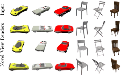
Figure 3:ShapeNet-SRN. Our method is able to represent difficult geometries (e.g., windshield in yellow car), and preserve details of the conditioning image (front of red car), occluded parts (left chair), thin structures (middle chair) and complex shapes (right chair).
图3：ShapeNet-SRN。我们的方法能够表示困难的几何形状（例如，黄色汽车的挡风玻璃），并保留调节图像（红色汽车的前部）、遮挡部分（左椅子）、薄结构（中间椅子）和复杂形状（右椅子）的细节。

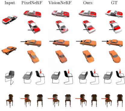
Figure 4:ShapeNet-SRN Comparison. Our method outputs more accurate reconstructions (cars’ backs, top chair) and better represents thin regions (bottom chair).
图4：ShapeNet-SRN比较。我们的方法输出更准确的重建（汽车的背部，顶部的椅子），更好地代表薄的地区（底部的椅子）。

CO3D. CO3D。

Qualitative results and a comparison to PixelNeRF are shown in Fig. 5. Splatter Image predicts sharper images while also being 1000× faster. Quantitatively (Tab. 2) our model outperforms PixelNeRF for both categories on SSIM and LPIPS and results in PSNR on par with PixelNeRF.
定性结果和与PixelNeRF的比较如图5所示。飞溅图像预测更清晰的图像，同时也是1000 × 快。定量（表2)我们的模型在SSIM和LPIPS两个类别上都优于PixelNeRF，并且导致与PixelNeRF相当的PSNR。

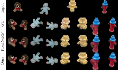
Figure 5:CO3D Hydrants and Teddybears. Our method outputs sharper reconstructions than PixelNeRF while being 100x faster in inference.
图5：CO3D消防栓和泰迪熊。我们的方法输出比PixelNeRF更清晰的重建，同时推理速度快100倍。

Object	Method	PSNR ↑	SSIM ↑	LPIPS ↓
Hydrant	PixelNeRF	21.76	0.78	0.207
Hydrant	Ours	22.10	0.81	0.148
Teddybear	PixelNeRF	19.57	0.67	0.297
Teddybear	Ours	19.51	0.73	0.236

Table 2:CO3D: Single-View. Our method outperforms PixelNeRF on this challenging benchmark across most metrics.
表2：CO 3D：单视图。我们的方法在大多数指标上都优于PixelNeRF。

4.1.2Two-view 3D reconstruction
4.1.2两视图三维重建

We compare our multi-view reconstruction model on ShapeNet-SRN Cars by training a model for two-view predictions (see Tab. 3). Prior work often relies on absolute camera pose conditioning, meaning that the model learns to rely on the canonical orientation of the object in the dataset. This limits the applicability of these models, as in practice for a new image of an object, the absolute camera pose is of course unknown. Here, only ours and PixelNeRF can deal with relative camera poses as input. Interestingly, our method shows not only better performance than PixelNeRF but also improves over SRN, CodeNeRF, and FE-NVS that rely on absolute camera poses.
我们通过训练一个双视图预测模型来比较我们在ShapeNet-SRN汽车上的多视图重建模型（见表1）。3）。以前的工作通常依赖于绝对相机姿态调节，这意味着模型学习依赖于数据集中对象的规范方向。这限制了这些模型的适用性，因为在实践中，对于对象的新图像，绝对相机姿态当然是未知的。在这里，只有我们的和PixelNeRF可以处理相对相机姿势作为输入。有趣的是，我们的方法不仅表现出比PixelNeRF更好的性能，而且还优于依赖于绝对相机姿势的SRN，CodeNeRF和FE-NVS。

Method	Relative	2-view Cars 2-查看汽车
	Pose	PSNR ↑	SSIM ↑
SRN	✗	24.84	0.92
CodeNeRF	✗	25.71	0.91
FE-NVS	✗	24.64	0.93
PixelNeRF	✓	25.66	0.94
Ours	✓	26.01	0.94

Table 3:Two-view reconstruction on ShapeNet-SRN Cars.
表3：ShapeNet-SRN汽车上的双视图重建。

4.1.3Ablations

We evaluate the influence of individual components of our method on the final performance. Due to computational cost, we train these models at a shorter training schedule for 100k iterations with ℒ2 and further 25k with ℒ2 and ℒLPIPS.
我们评估我们的方法的各个组成部分对最终性能的影响。由于计算成本，我们以较短的训练时间表训练这些模型，使用 ℒ2 进行100k次迭代，使用 ℒ2 和 ℒLPIPS 进行25k次迭代。

Single-View Model. 单视图模型。

We show the results of our ablation study for the single-view model in Tab. 4. We test the impact of all components. We train a model (w/o image) that uses a fully connected, unstructured output instead of a Splatter Image. This model cannot transfer image information directly to their corresponding Gaussians and does not achieve good performance. We also ablate predicting the depth along the ray by simply predicting 3D coordinates for each Gaussian. This version also suffers from its inability to easily align the input image with the output. Removing the 3D offset prediction mainly harms the backside of the object while leaving the front faces the same. This results in a lower impact on the overall performance of this component. Changing the degrees of freedom of the predicted covariance matrix to be isotropic or removing view-dependent appearance (by removing Spherical Harmonics prediction) also reduced the image fidelity. Finally, removing perceptual loss (w/o ℒLPIPS) results in a very small drop in PSNR but a significant worsening of LPIPS, indicating this loss is important for perceptual sharpness of reconstructions. Being able to use LPIPS in optimisation is a direct consequence of employing a fast-to-render representation and being able to render full images at training time.
我们在表中显示了单视图模型的消融研究结果。4.我们测试所有组件的影响。我们训练一个模型（无镜像），它使用完全连接的非结构化输出，而不是飞溅的镜像。该模型不能将图像信息直接转换为相应的高斯模型，性能不佳。我们还通过简单地预测每个高斯的3D坐标来预测沿着射线的深度沿着。该版本还遭受其无法容易地将输入图像与输出对齐的问题。去除3D偏移预测主要损害对象的背面，而保持正面不变。这导致对该组件的整体性能的影响较低。将预测协方差矩阵的自由度更改为各向同性或删除视图相关外观（通过删除球面谐波预测）也会降低图像保真度。 最后，去除感知损失（w/o ℒLPIPS ）导致PSNR的非常小的下降，但是LPIPS的显著恶化，表明这种损失对于重建的感知锐度是重要的。能够在优化中使用LPIPS是采用快速渲染表示并能够在训练时渲染完整图像的直接结果。

Multi-View Model. 多视图模型。

Table 5 ablates the multi-view model. We individually remove the multi-view attention blocks, the camera embedding and the warping component of the multi-view model and find that they all are important to achieve the final performance.
表5消融了多视图模型。我们分别删除多视图注意块，相机嵌入和多视图模型的扭曲组件，并发现它们都是重要的，以实现最终的性能。

Analysis. 分析.

Figure 6:Analysis. Splatter Images represent full 360∘ of objects by allocating background pixels to appropriate 3D locations (third row) to predict occluded elements like wheels (left) or chair legs (middle). Alternatively, it predicts offsets in the foreground pixels to represent occluded chair parts (right).
图6：分析。飞溅图像通过将背景像素分配到适当的3D位置（第三行）来预测被遮挡的元素（如轮子（左）或椅子腿（中）），从而表示完整的 360∘ 对象。或者，它预测前景像素中的偏移以表示被遮挡的椅子部分（右）。

In Fig. 6, we analyse how 3D information is stored inside a Splatter Image. Since all information is arranged in an image format, we can visualise each of the modalities: opacity, depth, and location offset. Pixels of the input image that belong to the object tend to describe their corresponding 3D structure, while pixels outside of the object wrap around to close the object on the back.
在图6中，我们分析了3D信息如何存储在飞溅图像中。由于所有信息都以图像格式排列，因此我们可以可视化每种形式：不透明度，深度和位置偏移。属于对象的输入图像的像素倾向于描述其对应的3D结构，而对象外部的像素环绕以在背面闭合对象。

	PSNR ↑	SSIM ↑	LPIPS ↓
Full model 完整模型	22.25	0.90	0.115
w/o image 无图像	20.60	0.87	0.152
w/o depth 无深度	21.21	0.88	0.145
w/o view dir. w/o视图目录。	21.77	0.89	0.121
isotropic	22.01	0.89	0.118
w/o offset 无偏移	22.06	0.90	0.119
w/o ℒLPIPS	22.22	0.89	0.141

Table 4:Ablations: Single-View Reconstruction.
表4：消融：单视图重建。

	PSNR ↑	SSIM ↑	LPIPS ↓
Full model 完整模型	24.11	0.92	0.087
w/o cross-view attn 无交叉视图属性	23.68	0.92	0.091
w/o cam embed 无凸轮嵌入	23.91	0.92	0.088
w/o warping 无翘曲	23.84	0.92	0.088

Table 5:Ablations: Multi-View Reconstruction.
表5：消融：多视图重建。

4.2Assessing efficiency 4.2评估效率

	RP	E ↓ E编号0#	R ↓ R编号0#	Forward ↓ 转发 ↓	Test ↓ 测试编号0#
NeRFDiff	✓	(0.031)	(0.0180)	(0.103)	(4.531)
FE-NVS	✗	(0.015)	(0.0032)	(0.028)	(0.815)
VisionNeRF	✓	0.008	2.4312	9.733	607.8
PixelNeRF	✓	0.003	1.8572	7.432	463.3
ViewsetDiff	✗	0.025	0.0064	0.051	1.625
Ours 2-view 我们的2视图	✓	0.030	0.0017	0.037	0.455
Ours 1-view	✓	0.026	0.0017	0.033	0.451

Table 6:Speed. Time required for image encoding (E), rendering (R), the ‘Forward’ time, indicative of train-time efficiency and the ‘Test’ time, indicative of test-time efficiency. Our method is the most efficient in both train and test time across open-source available methods and only requires relative camera poses. ‘RP’ indicates if a method can operate using only relative camera poses.
表6：速度。图像编码（E）、渲染（R）所需的时间、指示训练时间效率的“向前”时间和指示测试时间效率的“测试”时间。我们的方法在训练和测试时间上都是最有效的，并且只需要相对的相机姿势。“RP”指示方法是否可以仅使用相对相机姿势来操作。

One advantage of the Splatter Image is its training and test time efficiency, which we assess below.
Splatter Image的一个优点是它的训练和测试时间效率，我们在下面评估。

Test-time efficiency. 测试时间效率。

First, we assess the ‘Test’ time speed, i.e., the time it takes for the trained model to reconstruct an object and generate a certain number of images. We reference the evaluation protocol of the standard ShapeNet-SRN benchmark [35] and render 250 images at 1282 resolution.
首先，我们评估“测试”时间速度，即，训练模型重建物体并生成一定数量的图像所需的时间。我们参考了标准ShapeNet-SRN基准测试[35]的评估协议，并以 1282 分辨率渲染250张图像。

Assessing wall-clock time fairly is challenging as it depends on many factors. All measurements reported here are done on a single NVIDIA V100 GPU. We use officially released code of Viewset Diffusion [38], PixelNeRF [44] and VisionNeRF [16] and rerun those on our hardware. NeRFDiff [7] and FE-NVS [8] do not have code available, so we use their self-reported metrics. FE-NVS was evaluated ostensibly on the same type of GPU, while NeRFDiff does not include information about the hardware used and we were unable to obtain more information. Since we could not perfectly control these experiments, the comparisons to NeRFDiff and FE-NVS are only indicative. For Viewset Diffusion and NeRFDiff we report the time for a single pass through the reconstruction network.
公平地评估挂钟时间具有挑战性，因为它取决于许多因素。这里报告的所有测量都是在单个NVIDIA V100 GPU上完成的。我们使用官方发布的Viewset Diffusion [38]，PixelNeRF [44]和VisionNeRF [16]代码，并在我们的硬件上运行这些代码。NeRFDiff [7]和FE-NVS [8]没有可用的代码，所以我们使用他们的自我报告指标。FE-NVS表面上是在相同类型的GPU上进行评估的，而NeRFDiff不包括有关所使用硬件的信息，我们无法获得更多信息。由于我们无法完全控制这些实验，因此与NeRFDiff和FE-NVS的比较仅具有指示性。对于Viewset Diffusion和NeRFDiff，我们报告单次通过重建网络的时间。

Tab. 6 reports the ‘Encoding’ (E) time, spent by the network to compute the object’s 3D representation from an image, and the ‘Rendering’ (R) time, spent by the network to render new images from the 3D representation. From those, we calculate the ‘Test’ time, equal to the ‘Encoding’ time plus 250 ‘Rendering’ time. As shown in the last column of Tab. 6, our method is more than 1000× faster in testing than PixelNeRF and VisionNeRF (while achieving equal or superior quality of reconstruction in Tab. 1). Our method is also faster than voxel-based Viewset Diffusion even though does not require knowing the absolute camera pose. The efficiency of our method is very useful to iterate quickly in research; for instance, evaluating our method on the full ShapeNet-Car validation set takes less than 10 minutes on a single GPU. In contrast, PixelNeRF takes 45 GPU-hours.
选项卡. 6报告了网络从图像计算对象的3D表示所花费的“编码”（E）时间，以及网络从3D表示渲染新图像所花费的“渲染”（R）时间。从这些，我们计算'测试'时间，等于'编码'时间加上250 '渲染'时间。如Tab的最后一列所示。6，我们的方法在测试中比PixelNeRF和VisionNeRF快 1000× 以上（同时在Tab. 1）。我们的方法也比基于体素的视图集扩散更快，即使不需要知道绝对相机姿势。我们的方法的效率对于快速搜索研究非常有用;例如，在完整的ShapeNet-Car验证集上评估我们的方法在单个GPU上花费不到10分钟。相比之下，PixelNeRF需要45个GPU小时。

Train-time efficiency. 列车时间效率

Next, we assess the efficiency of the method during training. Here, the encoding time becomes more significant because one typically renders only a few images to compute the reconstruction loss and obtain a gradient (e.g., because there are only so many views available in the training dataset, or because generating more views provides diminishing returns in terms of supervision). As typical values (and as used by us in this work), we assume that the method is tasked with generating 4 new views at each iteration instead of 250 as before. We call this the ‘Forward’ time and measure it the same way. As shown in the ‘Forward’ column of Tab. 6, our method is 246× faster at training time than implicit methods and 1.5× than Viewset Diffusion, which uses an explicit representation. With this, we can train models achieving state-of-the-art quality on a single A6000 GPU in 7 days, while VisionNeRF requires 16 A100 GPUs for 5 days.
接下来，我们在训练过程中评估该方法的效率。这里，编码时间变得更加重要，因为通常仅渲染几个图像来计算重建损失并获得梯度（例如，因为在训练数据集中只有这么多视图可用，或者因为生成更多视图在监督方面提供了递减的回报）。作为典型值（以及我们在本工作中使用的值），我们假设该方法的任务是在每次迭代中生成4个新视图，而不是像以前那样生成250个视图。我们称之为“前进”时间，并以同样的方式测量它。如选项卡的“转发”列所示。6，我们的方法在训练时比隐式方法快 246× ，比使用显式表示的视图集扩散快 1.5× 。有了这个，我们可以在7天内在单个A6000 GPU上训练模型，达到最先进的质量，而VisionNeRF需要16个A100 GPU 5天。

5Conclusion 5结论

We have presented Splatter Image, a simple and fast method for single- or few-view 3D reconstruction. The method processes images efficiently using an off-the-shelf 2D CNN architecture and predicts a pseudo-image containing one colored 3D Gaussian per pixel. By combining fast inference with fast rendering via Gaussian Splatting, Splatter Image can be trained and evaluated quickly on synthetic and real benchmarks. Splatter Image achieves state-of-the-art performance, does not require canonical camera poses, is simple to implement and offers significant computational savings in both training and inference.
我们已经提出了飞溅图像，一个简单而快速的方法，单视图或少视图的三维重建。该方法使用现成的2D CNN架构有效地处理图像，并预测每个像素包含一个彩色3D高斯的伪图像。通过将快速推理与快速渲染相结合，通过高斯飞溅，飞溅图像可以在合成和真实的基准上快速训练和评估。Splatter Image实现了最先进的性能，不需要规范的相机姿势，易于实现，并在训练和推理中提供了显着的计算节省。