多合约日间趋势交易策略—机器学习策略——核密度估计与KNN

单一合约日间趋势交易策略—机器学习策略——核密度估计与KNN

核密度估计

直方图

$f(x)=\frac{n_x}{nh}$
其中， n x = # { 样本点落在包含 x 的区间内 } n_x=\#\{样本点落在包含x的区间内\} nx​=#{样本点落在包含x的区间内}，$h$为区间长度(带宽)，$n$为样本点个数

除以带宽$h$的原因：

已知$\sum _x\frac{n_x}{n}=1$
不除以带宽：矩形总面积为$S=\sum _{x}f(x)h=\sum _x\frac{n_x}{n}h=h$
除以带宽：矩形总面积为$S=\sum _{x}f(x)h=\sum _x\frac{n_x}{nh}h=1$

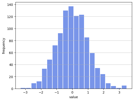
# 生成服从N(0,1)的随机数
import numpy as np
data = np.random.randn(1000)

# 绘制直方图
import matplotlib.pyplot as plt
plt.hist(data,bins=20,alpha=0.7,rwidth=0.9,color='royalblue')
plt.grid(axis='y',alpha=0.75)
plt.xlabel('value')
plt.ylabel('frequency')

核密度估计

核密度估计是在直方图的基础上进一步推导得出：
f ^ h ( x ) = 1 2 n h # { X i ∈ [ x − h , x + h ) } = 1 2 n h ∑ i = 1 n I { X i ∈ [ x − h , x + h ) } = 1 n h ∑ i = 1 n 1 2 I { − 1 ≤ X i − x h < 1 } = 1 n h ∑ i = 1 n 1 2 I { ∣ x − X i h ∣ ≤ 1 } = 1 n h ∑ i = 1 n K ( x − X i h ) = 1 n h ∑ i = 1 n K ( u ) ( u = x − X i h ) \begin{align*} \hat{f}_h(x)&=\dfrac{1}{2nh}\#\{X_i\in[x-h,x+h)\} \\ &=\dfrac{1}{2nh}\sum\limits_{i=1}^nI\{X_i\in[x-h,x+h)\} \\ &=\dfrac{1}{nh}\sum\limits_{i=1}^n\dfrac{1}{2}I\{-1\le\dfrac{X_i-x}{h}<1\} \\ &=\dfrac{1}{nh}\sum\limits_{i=1}^n\dfrac{1}{2}I\{|\dfrac{x-X_i}{h}|\le 1\} \\ &=\dfrac{1}{nh}\sum\limits_{i=1}^nK(\dfrac{x-X_i}{h}) \\ &=\dfrac{1}{nh}\sum\limits_{i=1}^nK(u)\quad(u=\dfrac{x-X_i}{h}) \end{align*} f^​h​(x)​=2nh1​#{Xi​∈[x−h,x+h)}=2nh1​i=1∑n​I{Xi​∈[x−h,x+h)}=nh1​i=1∑n​21​I{−1≤hXi​−x​<1}=nh1​i=1∑n​21​I{∣hx−Xi​​∣≤1}=nh1​i=1∑n​K(hx−Xi​​)=nh1​i=1∑n​K(u)(u=hx−Xi​​)​

核函数

Uniform K ( u ) = 1 2 I { ∣ u ∣ ≤ 1 } K(u)=\dfrac{1}{2}I\{|u|\le1\} K(u)=21​I{∣u∣≤1}

Triangle ( 1 − ∣ u ∣ ) I { ∣ u ∣ ≤ 1 } (1-|u|)I\{|u|\le1\} (1−∣u∣)I{∣u∣≤1}

Epanechnikov 3 4 ( 1 − u 2 ) I { ∣ u ∣ ≤ 1 } \dfrac{3}{4}(1-u^2)I\{|u|\le1\} 43​(1−u2)I{∣u∣≤1}

Quartic(Biweight) 15 16 ( 1 − u 2 ) 2 I { ∣ u ∣ ≤ 1 } \dfrac{15}{16}(1-u^2)^2I\{|u|\le1\} 1615​(1−u2)2I{∣u∣≤1}

Triweight 35 32 ( 1 − u 2 ) 3 I { ∣ u ∣ ≤ 1 } \dfrac{35}{32}(1-u^2)^3I\{|u|\le1\} 3235​(1−u2)3I{∣u∣≤1}

Gaussian $\frac{1}{\sqrt{2\pi }}exp(-\frac{1}{2}{u}^2)$

Cosine π 4 c o s ( π 2 u ) I { ∣ u ∣ ≤ 1 } \dfrac{\pi}{4}cos(\dfrac{\pi}{2}u)I\{|u|\le1\} 4π​cos(2π​u)I{∣u∣≤1}

代码与模拟

## 一维核密度估计
import numpy as np

def Kernerl_Density(X: np.array, x: np.array, h: float, kernel: str ='Uniform')->np.array:
    ''' 
    input:
        X: 样本点
        x: 待估点
        h: 带宽
        kernel: 核函数(Uniform, Triangle, Epanechnikov, Quartic, Triweight, Gaussian, Cosine)
    output:
        密度
    '''
    # 核函数
    def Kernel(u: float, kernel: str)->float:
        K = ['Uniform','Triangle','Epanechnikov','Quartic','Triweight','Cosine']
        K_ = [0.5, 1-np.abs(u), 0.75*(1-u**2), 15/16*(1-u**2)**2, 35/32*(1-u**2)**3, np.pi/4*np.cos(np.pi*u/2)]
        result = 0
        for i in range(len(K)):
            if kernel == K[i]:
                if np.abs(u) <= 1:
                    result = K_[i]
        if kernel == 'Gaussian':
            result = np.exp(-0.5*u**2)/(2*np.pi)**0.5
        return result
    
    n = len(X)
    f = np.zeros(len(x))
    for i in range(len(x)):
        u = (x[i]-X)/h
        K = np.zeros(n)
        for j in range(n):
            K[j] = Kernel(u[j], kernel)
        f[i] = np.sum(K)/(n*h)
    
    return f

## 绘图（折线图）
import numpy as np
import matplotlib.pyplot as plt
def plot(x: np.array, y: np.array, color: str = 'royalblue', alpha: float = 0.85, grid: 'str' = 'off', grid_alpha: float = 0.7):
    ''' 
    input:
        x: x轴的数据
        y: y轴的数据
        color: 颜色
        alpha: 透明度
        grid: 'on'所有网格线, 'off'关闭网格线, 'x'只打开x轴的网格线, 'y'只打开y轴的网格线
        grid_alpha: 网格线透明度
    '''
    plt.plot(x,y,color=color,alpha=alpha)
    if grid == 'on':
        plt.grid(alpha=grid_alpha)
    if (grid == 'x') | (grid == 'y'):
        plt.grid(axis=grid,alpha=grid_alpha)

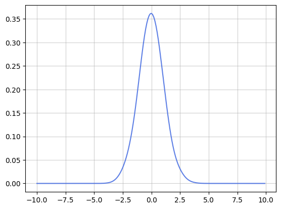
# 生成服从N(0,1)的随机数
import numpy as np
data = np.random.randn(1000)

import matplotlib.pyplot as plt
x = np.array([0.1*i for i in range(-100,100)])
f = Kernerl_Density(data,x,h=0.5,kernel='Gaussian')

plot(x,f,grid='on',grid_alpha=0.6)

累积分布函数推导与实现

公式推导

$$\begin{array}{rl}{\hat{F}}_h(t)& ={\int }_{-\infty }^t{\hat{f}}_h(x)dx\\ & ={\int }_{-\infty }^t\frac{1}{nh}\sum _{i=1}^{n}K(\frac{x-X_i}{h})dx\\ & =\frac{1}{nh}\sum _{i=1}^n{\int }_{-\infty }^{t}K(\frac{x-X_i}{h})dx\\ (u=\frac{x-X_i}{h})& =\frac{1}{nh}\sum _{i=1}^n{\int }_{-\infty }^{(t-X_i)/h}K(u)hdu\\ & =\frac{1}{n}\sum _{i=1}^n{\int }_{-\infty }^{(t-X_i)/h}K(u)du\end{array}$$

代码实现与模拟

## 累积分布函数（单个待估点的累积密度值）
from scipy import integrate
import numpy as np

def Kernel_Density_Cdf(X: np.array, x: np.array, h: float, kernel: str ='Uniform')->np.array:
    ''' 
    input:
        X: 样本点
        x: 待估点
        h: 带宽
        kernel: 核函数(Uniform, Triangle, Epanechnikov, Quartic, Triweight, Gaussian, Cosine)
    output:
        累积密度, 即<=x的概率
    '''
    # 核函数
    def Kernel1(u): # Uniform
        return 0.5
    def Kernel2(u): # Triangle
        return 1-np.abs(u)
    def Kernel3(u): # Epanechnikov
        return 0.75*(1-u**2)
    def Kernel4(u): # Quartic
        return 15/16*(1-u**2)**2
    def Kernel5(u): # Triweight
        return 35/32*(1-u**2)**3
    def Kernel6(u): # Gaussian
        return np.exp(-0.5*u**2)/(2*np.pi)**0.5
    def Kernel7(u): # Cosine
        return np.pi/4*np.cos(np.pi*u/2)
    
    n = len(X)
    U = np.zeros(n)
    # 核函数判断
    for i in range(n):  
        if kernel == 'Uniform':
            if -1 <= (x-X[i])/h <= 1:
                v, err = integrate.quad(Kernel1,-1,(x-X[i])/h)
                U[i] = v
            elif 1 <= (x-X[i])/h:
                v, err = integrate.quad(Kernel1,-1,1)
                U[i] = v
        elif kernel == 'Triangle':
            if -1 <= (x-X[i])/h <= 1:
                v, err = integrate.quad(Kernel2,-1,(x-X[i])/h)
                U[i] = v
            elif 1 <= (x-X[i])/h:
                v, err = integrate.quad(Kernel2,-1,1)
                U[i] = v
        elif kernel == 'Epanechnikov':
            if -1 <= (x-X[i])/h <= 1:
                v, err = integrate.quad(Kernel3,-1,(x-X[i])/h)
                U[i] = v
            elif 1 <= (x-X[i])/h:
                v, err = integrate.quad(Kernel3,-1,1)
                U[i] = v
        elif kernel == 'Quartic':
            if -1 <= (x-X[i])/h <= 1:
                v, err = integrate.quad(Kernel4,-1,(x-X[i])/h)
                U[i] = v
            elif 1 <= (x-X[i])/h:
                v, err = integrate.quad(Kernel4,-1,1)
                U[i] = v
        elif kernel == 'Triweight':
            if -1 <= (x-X[i])/h <= 1:
                v, err = integrate.quad(Kernel5,-1,(x-X[i])/h)
                U[i] = v
            elif 1 <= (x-X[i])/h:
                v, err = integrate.quad(Kernel5,-1,1)
                U[i] = v
        elif kernel == 'Gaussian':
            v, err = integrate.quad(Kernel6,-np.inf,(x-X[i])/h)
            U[i] = v
        elif kernel == 'Cosine':
            if -1 <= (x-X[i])/h <= 1:
                v, err = integrate.quad(Kernel7,-1,(x-X[i])/h)
                U[i] = v
            elif 1 <= (x-X[i])/h:
                v, err = integrate.quad(Kernel7,-1,1)
                U[i] = v
    F = np.sum(U)/n
    
    return F

## 累积分布函数绘图（多个待估点的累积密度值）
from scipy import integrate
import numpy as np

def Kernel_Density_Cdf_plot(X: np.array, x: np.array, h: float, kernel: str ='Uniform')->np.array:
    ''' 
    input:
        X: 样本点
        x: 待估点
        h: 带宽
        kernel: 核函数(Uniform, Triangle, Epanechnikov, Quartic, Triweight, Gaussian, Cosine)
    output:
        累积密度, 即<=x的概率
    '''
    # 核函数
    def Kernel1(u): # Uniform
        return 0.5
    def Kernel2(u): # Triangle
        return 1-np.abs(u)
    def Kernel3(u): # Epanechnikov
        return 0.75*(1-u**2)
    def Kernel4(u): # Quartic
        return 15/16*(1-u**2)**2
    def Kernel5(u): # Triweight
        return 35/32*(1-u**2)**3
    def Kernel6(u): # Gaussian
        return np.exp(-0.5*u**2)/(2*np.pi)**0.5
    def Kernel7(u): # Cosine
        return np.pi/4*np.cos(np.pi*u/2)
    
    n = len(X)
    F = np.zeros(len(x))
    for j in range(len(x)):
        U = np.zeros(n)
        # 核函数判断
        for i in range(n):  
            if kernel == 'Uniform':
                if -1 <= (x[j]-X[i])/h <= 1:
                    v, err = integrate.quad(Kernel1,-1,(x[j]-X[i])/h)
                    U[i] = v
                elif 1 <= (x[j]-X[i])/h:
                    v, err = integrate.quad(Kernel1,-1,1)
                    U[i] = v
            elif kernel == 'Triangle':
                if -1 <= (x[j]-X[i])/h <= 1:
                    v, err = integrate.quad(Kernel2,-1,(x[j]-X[i])/h)
                    U[i] = v
                elif 1 <= (x[j]-X[i])/h:
                    v, err = integrate.quad(Kernel2,-1,1)
                    U[i] = v
            elif kernel == 'Epanechnikov':
                if -1 <= (x[j]-X[i])/h <= 1:
                    v, err = integrate.quad(Kernel3,-1,(x[j]-X[i])/h)
                    U[i] = v
                elif 1 <= (x[j]-X[i])/h:
                    v, err = integrate.quad(Kernel3,-1,1)
                    U[i] = v
            elif kernel == 'Quartic':
                if -1 <= (x[j]-X[i])/h <= 1:
                    v, err = integrate.quad(Kernel4,-1,(x[j]-X[i])/h)
                    U[i] = v
                elif 1 <= (x[j]-X[i])/h:
                    v, err = integrate.quad(Kernel4,-1,1)
                    U[i] = v
            elif kernel == 'Triweight':
                if -1 <= (x[j]-X[i])/h <= 1:
                    v, err = integrate.quad(Kernel5,-1,(x[j]-X[i])/h)
                    U[i] = v
                elif 1 <= (x[j]-X[i])/h:
                    v, err = integrate.quad(Kernel5,-1,1)
                    U[i] = v
            elif kernel == 'Gaussian':
                v, err = integrate.quad(Kernel6,-np.inf,(x[j]-X[i])/h)
                U[i] = v
            elif kernel == 'Cosine':
                if -1 <= (x[j]-X[i])/h <= 1:
                    v, err = integrate.quad(Kernel7,-1,(x[j]-X[i])/h)
                    U[i] = v
                elif 1 <= (x[j]-X[i])/h:
                    v, err = integrate.quad(Kernel7,-1,1)
                    U[i] = v
        F[j] = np.sum(U)/n
    
    return F
    

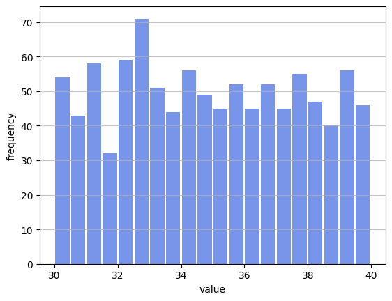
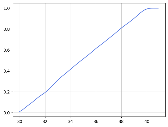
模拟如下：生成数据后分别绘制直方图、核密度曲线图、核密度累积分布图

# 生成1000个随机数
import numpy as np
data = 30+10*np.random.rand(1000)

# 绘制直方图
import matplotlib.pyplot as plt
plt.hist(data,bins=20,alpha=0.7,rwidth=0.9,color='royalblue')
plt.grid(axis='y',alpha=0.75)
plt.xlabel('value')
plt.ylabel('frequency')

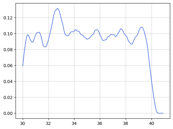
# 绘制核密度曲线
f = Kernerl_Density(data,x,h=0.5,kernel='Epanechnikov')
plot(x,f,grid='on',grid_alpha=0.6)

# 绘制核密度的累积分布曲线
x = np.array([0.1*i for i in range(300,410)])
F = Kernel_Density_Cdf_plot(data,x,h=0.5,kernel='Epanechnikov')
plot(x,F,grid='on',grid_alpha=0.6)

K近邻思想

我们这里仅仅参考K近邻的思想，采用欧式距离找到离我们的目标样本点最近的100个点，并对这100个点进一步进行分析。
以下我们设计一个函数以供后面进行实现以寻找最近的点。

# 借助KNN思想，找到最近的100个点
import numpy as np
def Knn(X: np.array, Y: np.array, x: np.array, k: int=100)->np.array:
    ''' 
    input:
        X,Y: 训练数据集, X每1行为1个样本点, 
        x: 待估点
        k: 选择最近的k个点
    output:
    '''
    # 欧式距离
    def dist(x1,x2):
        return (np.sum((x1-x2)**2))**0.5
    
    # 训练集所有点离待估点的欧式距离
    d = np.zeros(len(X))
    for i in range(len(X)):
        d[i] = dist(X[i],x)
    d = list(d)
    
    # 距离最近的k个点的索引
    Index = np.zeros(k,dtype=int)
    for i in range(k):
        index = d.index(min(d)) # 选取距离最近的点的索引
        Index[i] = index
        d[index] = np.inf # 选取过的点其距离值设为无穷大，防止再被选中
    
    y = Y[Index]
    return y

## 函数调用方法举例
X = np.random.randn(1000,2)
Y = np.random.rand(1000)
x = np.random.randn(1)

y = Knn(X,Y,x)

逻辑过程

参照在单均线策略中拟好的框架

既然在之前的单均线和双均线策略中，我们都是利用过去的数据来对未来趋势做出判断，即预测合约价格在隔天的涨跌情况。对于这种回归或分类预测问题，在机器学习中有诸多方法与模型去拟合，但所训练模型的泛化能力很大程度上取决是提取的特征是否有效、以及数据量是否充足。

将机器学习运用于CTA策略确实是一件蛮有诱惑力的事情，但针对日频交易策略，一份合约从其上市期到交割期，数据量比较缺乏，这将是我们亟需解决的第一个问题。

那么我们可以怎么寻找数据呢，笔者首先可以联想到股指期货主力合约（主连），主连的优点在于没有周期，数据量充足，由合约中成交量最大的合约的K线连成。简单举个例子来说，当中证500主连的标的合约是中证500的6月份当月合约时，其两者的价格是相同的。

也就是说，当主连上涨时，标的同样上涨，下跌时也同理，那我们便可以把预测标的合约涨跌转换为预测主连涨跌，当预测主连隔天价格上涨时，做多对应的合约标的，当预测主连隔天价格下跌时，对应地做空对应的合约标的。

那么，我们可以将策略（回测框架）初步设置如下：

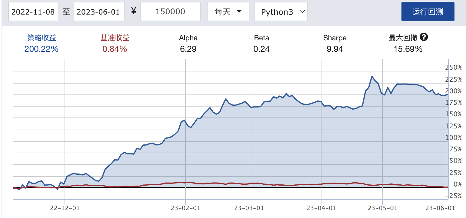
1. 回测时间为2022年11月8日至2023年6月1日，故我们先获取中证500主力合约于2022年11月7日过去3000个交易日的开盘价数据。
2. 特征提取：我们定义如下10个特征：当日开盘价涨跌（涨为1，跌为0）为第1个特征，昨日开盘价涨跌（涨为1，跌为0）为第2个特征，如此提取下去，直到有10个特征为止；另外将标签设置为隔天开盘价。这样设置的目的是把过去的涨跌与未来的价格对应起来。
3. 基于KNN思想寻找离当日最近的200个样本点，并记录下这200个样本点对应的标签值，即在过去的信息中，找到前10天涨跌趋势与当日的前10天涨跌趋势最相似的200个样本点。
4. 对这200个样本点对应的标签值，利用核密度估计刻画其分布，并用推导的核密度估计累积分布函数，去计算高于当天的开盘价的概率。
5. 当概率>0.5时，说明隔天开盘价上涨的可能性较大，那我们便在当天开盘时进行做多主力合约对应的合约标的，并在隔天开盘时予以平仓；当概率<0.5时，说明隔天开盘价下跌的可能性较大，那我们便在当天开盘时进行做空主力合约对应的合约标的，并在隔天开盘时予以平仓。

为了简单表达策略的过程，我们将先针对2023年5月1日至2023年5月31日于本地进行代码实现与分析，后续再将完整的过程在JoinQuant上进行回测分析。

获取数据

我们首先利用聚宽分别获取中证500主连2022年11月7日之前3000个交易日的开盘价数据、中证500主连2023年2月28日往前30个交易日的开盘价数据、中证500主连在2023年2月31日对应的合约标的在2023年2月28日往前20个交易日的开盘价数据、中证500主连在2023年2月28日对应的合约标的在2023年2月28日往前20个交易日的结算价数据（注：以下代码需要在JoinQuant的研究环境下运行）

之所以要获取中证500主连2023年2月28日往前30个交易日的开盘价数据，比后面两组数据多10个交易日，是因为在提取特征时，我们还需要往前10天的数据。

df_train = get_bars('IC9999.CCFX', count=3000, unit='1d',end_dt='2022-11-07',include_now=True, fields=['date','open'], df=True)
df_train.set_index('date', inplace=True)
df_train.index.name = None
df_train.to_excel('中证500主连.xlsx')
df_train.head()

df_pred = get_bars('IC9999.CCFX', count=30, unit='1d',end_dt='2023-03-01',include_now=False, fields=['date','open'], df=True)
df_pred.set_index('date', inplace=True)
df_pred.index.name = None
df_pred.to_excel('中证500主连_预测.xlsx')
df_pred.head()

IC_trade = get_dominant_future('IC',date='2023-03-01')
df_trade1 = get_bars(IC_trade, count=20, unit='1d',include_now=False,end_dt='2023-03-01', fields=['date','open'], df=True)
df_trade1.set_index('date', inplace=True)
df_trade1.index.name = None
df_trade1.to_excel('中证500主连标的_开盘价.xlsx')
df_trade1.head()

df_trade2 = get_extras('futures_sett_price',IC_trade,count=20,end_date='2023-02-28',df=True)
df_trade2.to_excel('中证500主连标的_结算价.xlsx')
df_trade2.head()

策略构建

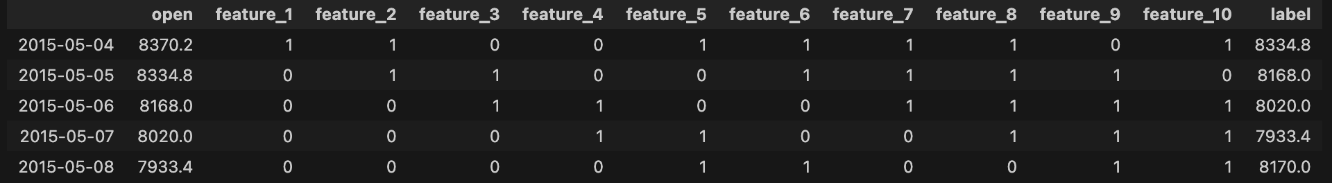
df1 = df_1.copy(deep=True)
t = 10
for i in range(1,t+1):
    df1['feature_'+str(i)] = np.where(df1['open'].shift(i-1)>df1['open'].shift(i),1,0)
df1['label'] = df1['open'].shift(-1)
df1.dropna(inplace=True)
df1.drop(df1.head(t).index,inplace=True)
df1.head()

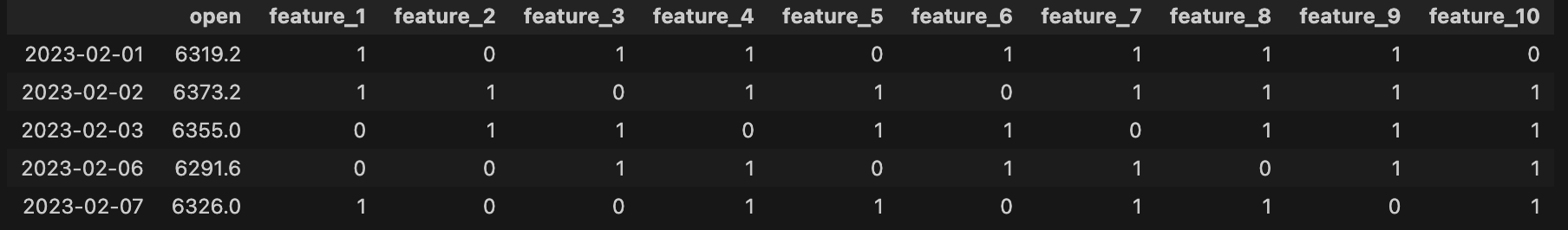
df2 = df_2.copy(deep=True)
t = 10
for i in range(1,t+1):
    df2['feature_'+str(i)] = np.where(df2['open'].shift(i-1)>df2['open'].shift(i),1,0)
df2.drop(df2.head(t).index,inplace=True)
df2.head()

X = np.array(df1.iloc[:,1:-1])
Y = np.array(df1.iloc[:,-1])
kernel = 'Epanechnikov'
k = 200
h = 0.5

prob = np.zeros(len(df2))
for i in range(len(df2)):
    x = df2.iloc[i,1:]
    y = Knn(X,Y,x)
    x_ = df2['open'][i]
    F = Kernel_Density_Cdf(y,x_,h=h,kernel=kernel)
    prob[i] = 1-F

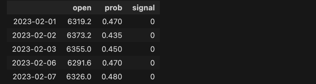
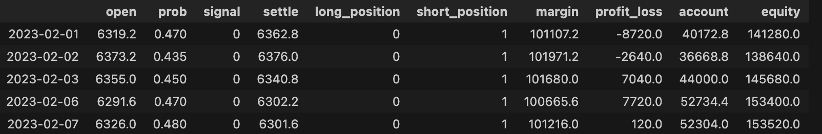
strat = pd.DataFrame()
strat.index = df2.index

strat['open'] = df_3['open']
strat['prob'] = prob
strat['signal'] = np.where(strat['prob']>0.5,1,0)
strat.head()

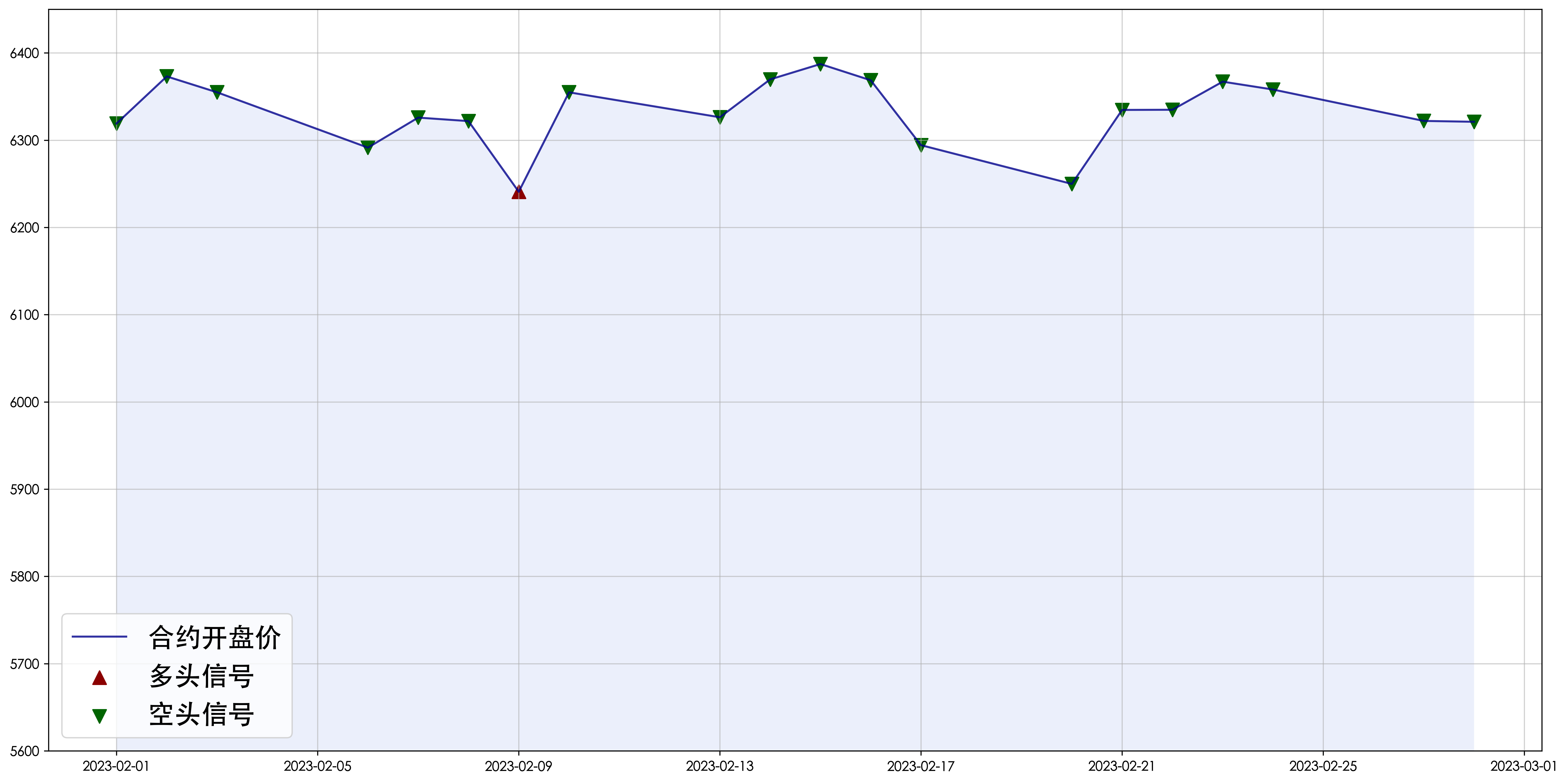
信号图

import matplotlib.pyplot as plt
# 设置画布，像素调高
plt.figure(figsize=(20,10),dpi=400)
# 解决中文显示问题
plt.rcParams['font.sans-serif']=['Heiti TC']

# 折线图
plt.plot(strat['open'],color='darkblue',alpha=0.8,label='合约开盘价')
plt.fill_between(x=strat.index, y1=5600, y2=strat['open'], facecolor='royalblue', alpha=0.1) # 折线下部填充
plt.ylim(5600,6450) # y轴范围
plt.grid(alpha=0.6) # 网格
# 散点图
plt.scatter(strat['open'][strat['signal']==1].index, strat['open'][strat['signal']==1], marker='^', c='darkred', s=100, label='多头信号')
plt.scatter(strat['open'][strat['signal']==0].index, strat['open'][strat['signal']==0], marker='v', c='darkgreen', s=100, label='空头信号')
plt.legend(fontsize=20) # 图例

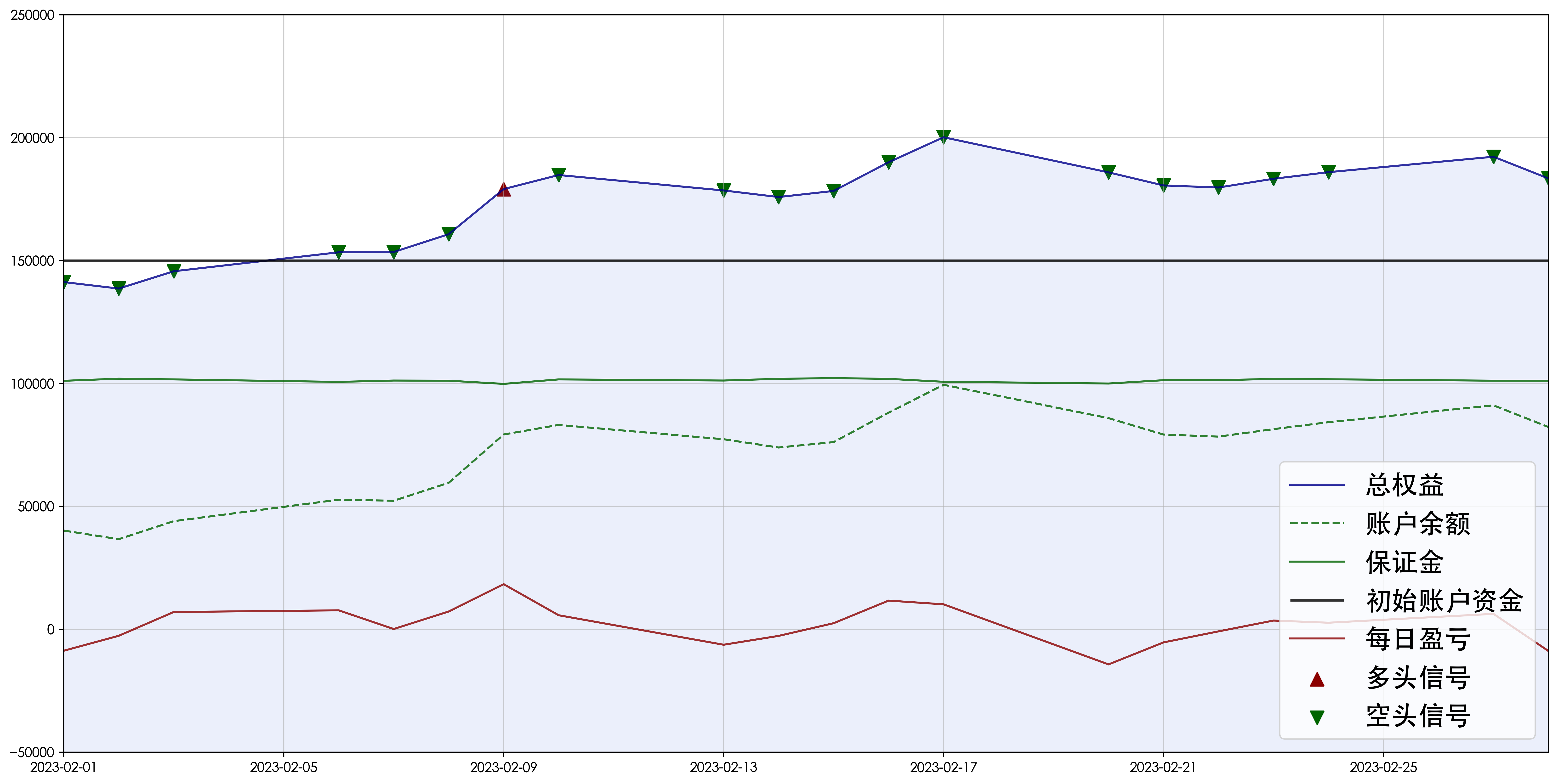
回测图

import warnings
warnings.filterwarnings("ignore")

# 账户初始资金15万
initial_cash = 150000 

strat['settle'] = df_4['IC2303.CCFX']
# 添加多头头寸字段'long_position'
strat['long_position'] = strat['signal']
# 添加空头头寸字段'short_position'
strat['short_position'] = np.where(strat['signal']==0, 1, 0)

multiplier = 200
margin_level = 0.08
num = 1
# 添加保证金字段'magin'
strat['margin'] = multiplier*strat['open']*num*margin_level
# 添加每日盈亏字段'profit_loss'
strat['profit_loss'] = (strat['open']-strat['settle'].shift(1))*multiplier*num + (strat['settle']-strat['open'])*multiplier*num
strat['profit_loss'][0] = (strat['settle'][0]-strat['open'][0])*multiplier*num
strat['profit_loss'][strat['signal']==0] = -1*strat['profit_loss'][strat['signal']==0]
# 增加账户资金余额字段'account'
strat['account'] = initial_cash-strat['margin']+strat['profit_loss'].cumsum()
# 增加总权益字段'equity'
strat['equity'] = strat['account']+strat['margin']

strat.head()

# 画布大小，调高像素
plt.figure(figsize=(20,10),dpi=400)
# 解决中文显示问题
plt.rcParams['font.sans-serif']=['Heiti TC']

plt.plot(strat['equity'],c='darkblue',alpha=0.8,label='总权益')
plt.plot(strat['account'],c='darkgreen',alpha=0.8,ls='--',label='账户余额')
plt.plot(strat['margin'],c='darkgreen',alpha=0.8,label='保证金')
plt.hlines(y=initial_cash,xmin=strat.index[0],xmax=strat.index[-1],color='k',lw=2,alpha=0.8,label='初始账户资金')
plt.plot(strat['profit_loss'],c='darkred',alpha=0.8,label='每日盈亏')

plt.scatter(strat['equity'][strat['signal']==1].index, strat['equity'][strat['signal']==1], marker='^', c='darkred', s=100, label='多头信号')
plt.scatter(strat['equity'][strat['signal']==0].index, strat['equity'][strat['signal']==0], marker='v', c='darkgreen', s=100, label='空头信号')

plt.fill_between(x=strat.index, y1=-50000, y2=strat['equity'], facecolor='royalblue', alpha=0.1) # 折线下部填充
plt.ylim(-50000,250000) # y轴范围
plt.xlim(strat.index[0],strat.index[-1])
plt.legend(fontsize=20)
plt.grid(alpha=0.6)

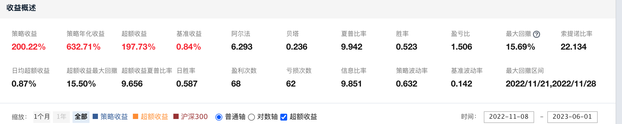
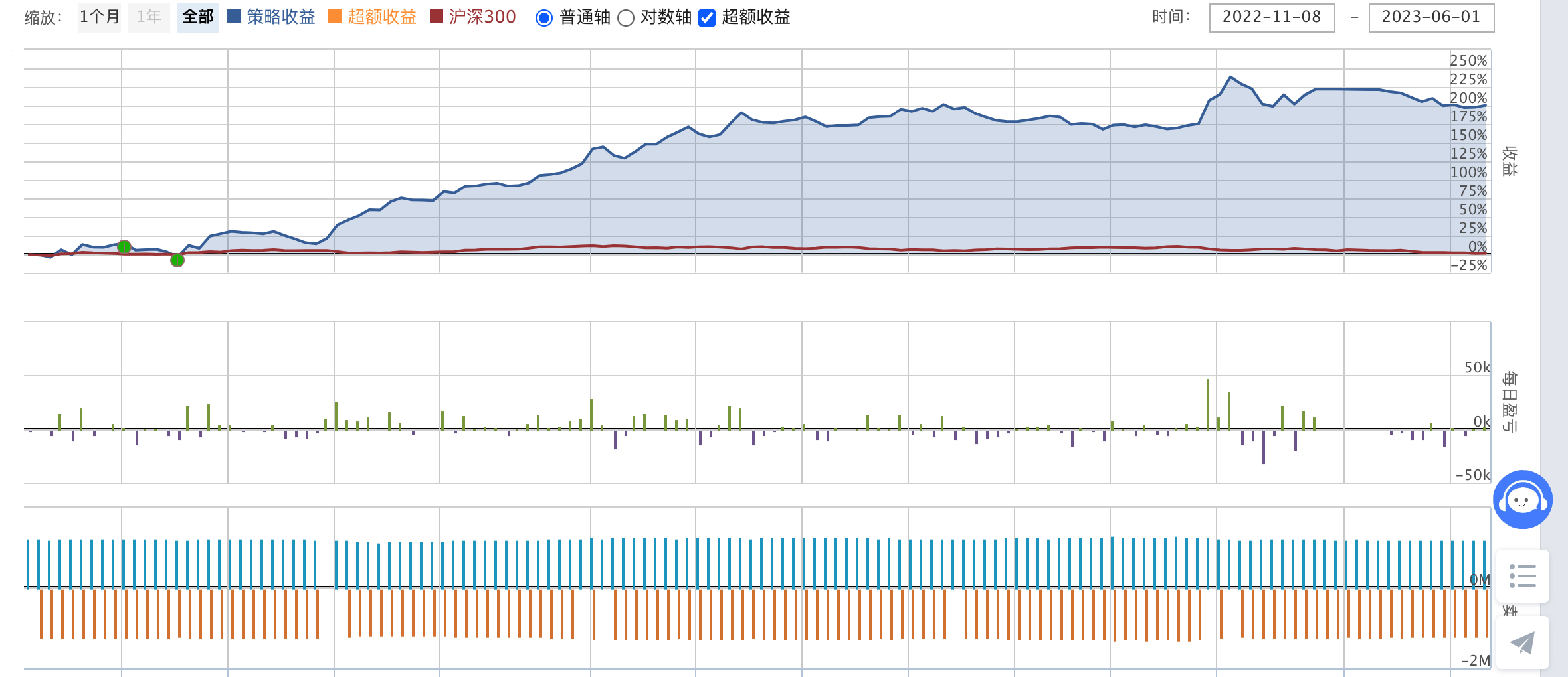
JoinQuant回测

(注：以下代码需在JoinQuant回测环境中运行）

# 导入函数库
from jqdata import *

## 初始化函数，设定基准等等
def initialize(context):
    # 设定沪深300作为基准
    set_benchmark('000300.XSHG')
    # 开启动态复权模式(真实价格)
    set_option('use_real_price', True)
    ### 期货相关设定 ###
    # 设定账户为金融账户
    set_subportfolios([SubPortfolioConfig(cash=context.portfolio.starting_cash, type='index_futures')])
    # 期货类每笔交易时的手续费是：买入时万分之0.23,卖出时万分之0.23,平今仓为万分之23
    set_order_cost(OrderCost(open_commission=0.000023, close_commission=0.000023,close_today_commission=0.0023), type='index_futures')
    # 设定保证金比例
    set_option('futures_margin_rate', 0.08)

    # 设置期货交易的滑点
    set_slippage(StepRelatedSlippage(2))
    # 开盘前运行
    run_daily( before_market_open, time='09:00', reference_security='IC9999.CCFX')
    # 开盘时运行
    run_daily( market_open, time='09:30', reference_security='IC9999.CCFX')
    # 收盘后运行
    run_daily( after_market_close, time='15:30', reference_security='IC9999.CCFX')


## 开盘前运行函数
def before_market_open(context):
    # 输出运行时间
    log.info('函数运行时间(before_market_open)：'+str(context.current_dt.time()))

    ## 选取要操作的合约(g.为全局变量)
    # 当天中证500主力合约所对应的合约标的（交易所用）
    g.IC_trade = get_dominant_future('IC')
    # 中证500主力合约IC9999.CCFX（训练与预测所用）
    g.IC_train = 'IC9999.CCFX'

## 开盘时运行函数
def market_open(context):
    log.info('函数运行时间(market_open):'+str(context.current_dt.time()))

    # 获取主力合约最近3000天的开盘价
    df_train = get_bars(g.IC_train, count=3000, unit='1d',end_dt='2022-11-07',include_now=True, fields=['date','open'], df=True)
    df_train.set_index('date', inplace=True)
    df_train.index.name = None
    
    df_test = get_bars(g.IC_train, count=11, unit='1d', include_now=True, fields=['date','open'],df=True)
    def strat(df_train,df_test,k,t,h,kernel):
        # df_train: 训练数据框
        # df_test: 预测数据框
        # k: Knn参数
        # t: 特征数,过往1到t天的收盘价作为特征
        # h: 核密度带宽
        # kernel: 核函数
        
        df1 = df_train.copy(deep=True)
        for i in range(1,t+1):
            df1['feature_'+str(i)] = np.where(df1['open'].shift(i-1)>df1['open'].shift(i),1,0)
        df1['label'] = df1['open'].shift(-1)
        df1.dropna(inplace=True)
        df1.drop(df1.head(10).index,inplace=True)
        
        x=np.zeros(t)
        for i in range(t):
            if df_test['open'][t-i] > df_test['open'][t-i-1]:
                x[i] = 1
        
        X = np.array(df1.iloc[:,1:-1])
        Y = np.array(df1.iloc[:,-1])
        y = Knn(X,Y,x,k)
        y_ = np.array(df_test['open'][-1:])
        F = Kernel_Density_Cdf(y,y_,h,kernel=kernel)
        prob = 1-F
        
        return prob
        
    k = 200
    t = 10
    h = 0.5 # 核密度估计带宽
    kernel = 'Epanechnikov' # 核密度估计核函数
    prob = strat(df_train,df_test,k,t,h,kernel)
    print(prob)

    
    # 获取当月合约交割日期
    end_data = get_security_info(g.IC_trade).end_date
    if (context.current_dt.date() == end_data):
        # return
        pass
    else:
        if (len(context.portfolio.short_positions) != 0):
            order_target(g.IC_trade, 0, side='short')
        if (len(context.portfolio.long_positions) != 0):
            order_target(g.IC_trade, 0, side='long')
        
        if prob>0.5:
            order(g.IC_trade, 1, side='long')
        elif prob<0.5:
            order(g.IC_trade, 1, side='short')
    

## 收盘后运行函数
def after_market_close(context):
    log.info(str('函数运行时间(after_market_close):'+str(context.current_dt.time())))
    # 得到当天所有成交记录
    trades = get_trades()
    for _trade in trades.values():
        log.info('成交记录：'+str(_trade))
    log.info('一天结束')
    log.info('##############################################################')

#########################自定义函数##################################
# 借助KNN思想，找到最近的200个点
import numpy as np
def Knn(X: np.array, Y: np.array, x: np.array, k: int=200)->np.array:
    ''' 
    input:
        X,Y: 训练数据集
        x: 待估点
        k: 选择最近的k个点
    output:
    '''
    
    def dist(x1,x2):
        return (np.sum((x1-x2)**2))**0.5
    
    d = np.zeros(len(X))
    for i in range(len(X)):
        d[i] = dist(X[i],x)
    d = list(d)
    
    Index = np.zeros(k,dtype=int)
    for i in range(k):
        index = d.index(min(d))
        Index[i] = index
        d[index] = np.inf
    
    y = Y[Index]
    return y

## 一维核密度的累积分布函数
from scipy import integrate
import numpy as np

def Kernel_Density_Cdf(X: np.array, x: np.array, h: float, kernel: str ='Uniform')->np.array:
    ''' 
    input:
        X: 样本点
        x: 待估点
        h: 带宽
        kernel: 核函数(Uniform, Triangle, Epanechnikov, Quartic, Triweight, Gaussian, Cosine)
    output:
        累积密度, 即<=x的概率
    '''
    
    def Kernel1(u): # Uniform
        return 0.5
    def Kernel2(u): # Triangle
        return 1-np.abs(u)
    def Kernel3(u): # Epanechnikov
        return 0.75*(1-u**2)
    def Kernel4(u): # Quartic
        return 15/16*(1-u**2)**2
    def Kernel5(u): # Triweight
        return 35/32*(1-u**2)**3
    def Kernel6(u): # Gaussian
        return np.exp(-0.5*u**2)/(2*np.pi)**0.5
    def Kernel7(u): # Cosine
        return np.pi/4*np.cos(np.pi*u/2)
    
    n = len(X)
    U = np.zeros(n)
    for i in range(n):  
        if kernel == 'Uniform':
            if -1 <= (x-X[i])/h <= 1:
                v, err = integrate.quad(Kernel1,-1,(x-X[i])/h)
                U[i] = v
            elif 1 <= (x-X[i])/h:
                v, err = integrate.quad(Kernel1,-1,1)
                U[i] = v
        elif kernel == 'Triangle':
            if -1 <= (x-X[i])/h <= 1:
                v, err = integrate.quad(Kernel2,-1,(x-X[i])/h)
                U[i] = v
            elif 1 <= (x-X[i])/h:
                v, err = integrate.quad(Kernel2,-1,1)
                U[i] = v
        elif kernel == 'Epanechnikov':
            if -1 <= (x-X[i])/h <= 1:
                v, err = integrate.quad(Kernel3,-1,(x-X[i])/h)
                U[i] = v
            elif 1 <= (x-X[i])/h:
                v, err = integrate.quad(Kernel3,-1,1)
                U[i] = v
        elif kernel == 'Quartic':
            if -1 <= (x-X[i])/h <= 1:
                v, err = integrate.quad(Kernel4,-1,(x-X[i])/h)
                U[i] = v
            elif 1 <= (x-X[i])/h:
                v, err = integrate.quad(Kernel4,-1,1)
                U[i] = v
        elif kernel == 'Triweight':
            if -1 <= (x-X[i])/h <= 1:
                v, err = integrate.quad(Kernel5,-1,(x-X[i])/h)
                U[i] = v
            elif 1 <= (x-X[i])/h:
                v, err = integrate.quad(Kernel5,-1,1)
                U[i] = v
        elif kernel == 'Gaussian':
            v, err = integrate.quad(Kernel6,-np.inf,(x-X[i])/h)
            U[i] = v
        elif kernel == 'Cosine':
            if -1 <= (x-X[i])/h <= 1:
                v, err = integrate.quad(Kernel7,-1,(x-X[i])/h)
                U[i] = v
            elif 1 <= (x-X[i])/h:
                v, err = integrate.quad(Kernel7,-1,1)
                U[i] = v
    F = np.sum(U)/n
    
    return F