udacity Markov定位 - python版本（2）

udacity Markov定位程序，实现观察模式定位，并最终实现完整定位。python版本，根据网上的C++程序改写，方便大家参考。

参考代码：

（1）https://github.com/informramiz?page=5&tab=repositories

这个工程项目里有代码以及数据。感谢作者的无私分享。

参考文章：

（1）自动驾驶定位算法(九)-直方图滤波定位-腾讯云开发者社区-腾讯云

这篇文章对于理解Bayes滤波很有帮助。

参考公式：

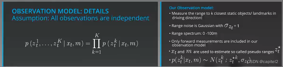
一、观察模式

本程序实现Markov定位中的观察模式。

二、车辆观察方式

车辆的传感器实现观察。车辆在实现移动到新的位置后，观察周边环境。

如下图示：

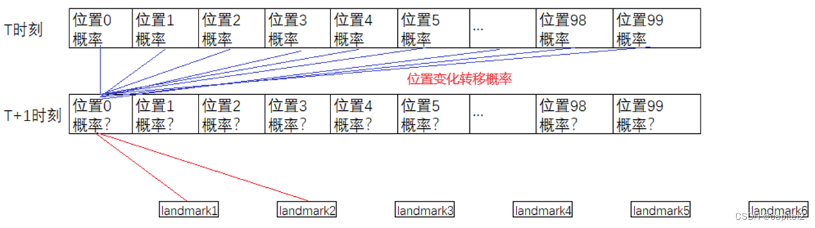
图1：观察模式

如上图示，车辆在某位置可以观察到landmark1，landmark2；也可以不进行观察。

三、数据说明

（1）地图数据

map_1d = [[1,9],[2,15],[3,25],[4,31],[5,59],[6,77]] 

（2）移动控制数据

controls_data = [1, 1, 1, 1, 1, 1, 1, 1, 1, 1, 1, 1, 1, 1]

车辆一次移动1米。

（3）观察数据

observations_data = [[1, 4.5], [2, -1], [3, -1], [4, -1], [5, -1], [6, -1], [7, 28], [8, 27], [9, 26], [10, 25], [11, -1], [12, -1], [13, -1], [14, -1]]
observations_data2 = [[1, 4.5], [1, 13.5], [2, -1], [3, -1], [4, -1], [5, -1], [6, -1], [7, 28], [8, 27], [9, 26], [10, 25], [11, -1], [12, -1], [13, -1], [14, -1]]
observations_data3 = [[1, 4.5], [1, 13.5], [2, -1], [3, -1], [4, -1], [5, -1], [6, -1], [7, 28], [8, 27], [9, 26], [10, 25], [11, -1], [12, -1], [13, -1], [14, 21]]
observations_data4 = [[1, 4.5], [1, 13.5], [2, -1], [3, -1], [4, -1], [5, -1], [6, -1], [7, 28], [8, 27], [9, 26], [10, 25], [11, -1], [12, -1], [13, -1], [14, 21],[14,30]]

observations_data，说明1,7,8,9,10时刻观察到路标，且每次只观察到1个路标。

observations_data2，说明1,7,8,9,10时刻观察到路标，1时刻观察到了2个路标；

observations_data3，说明1,7,8,9,10,14时刻观察到路标，1时刻观察到2个路标；

observations_data4，说明1,7,8,9,10,14时刻观察到路标，1,14时刻观察到2个路标。

四、Markov定位程序--包含移动模式+观察模式

import numpy as np
import matplotlib.pyplot as plt

class MeasurementPackage:
    def __init__(self,delta_x_f,obs):
        self.delta_x_f = delta_x_f
        self.observation_s_ = obs

b_initialized = 0
map_1d = [[1,9],[2,15],[3,25],[4,31],[5,59],[6,77]] #index,xf
controls_data = [1, 1, 1, 1, 1, 1, 1, 1, 1, 1, 1, 1, 1, 1]
observations_data = [[1, 4.5], [2, -1], [3, -1], [4, -1], [5, -1], [6, -1], [7, 28], [8, 27],             [9, 26], [10, 25], [11, -1], [12, -1], [13, -1], [14, -1]]
observations_data2 = [[1, 4.5], [1, 13.5], [2, -1], [3, -1], [4, -1], [5, -1], [6, -1], [7, 28], [8, 27],
              [9, 26], [10, 25], [11, -1], [12, -1], [13, -1], [14, -1]]
observations_data3 = [[1, 4.5], [1, 13.5], [2, -1], [3, -1], [4, -1], [5, -1], [6, -1], [7, 28], [8, 27],
              [9, 26], [10, 25], [11, -1], [12, -1], [13, -1], [14, 21]]
observations_data4 = [[1, 4.5], [1, 13.5], [2, -1], [3, -1], [4, -1], [5, -1], [6, -1], [7, 28], [8, 27],
              [9, 26], [10, 25], [11, -1], [12, -1], [13, -1], [14, 21],[14,30]]


bel_x_init = np.zeros(100)
bel_x = np.zeros(100)

M_PI = 3.1415926
ONE_OVER_SQRT_2PI = 1 / np.sqrt(2 * M_PI)
control_std = 1.0
observation_std = 1.0
distance_max = 100

measurement_elem = MeasurementPackage([], [])
measurement_pack_list = []

def square(x):
    return x * x

def normpdf(x, mu, std):
    return (ONE_OVER_SQRT_2PI / std) * np.exp(-0.5 * square((x - mu) / std))

def process_measurement(MeasurementPackage):
    global b_initialized
    global bel_x_init
    global bel_x
    if(b_initialized == 0):
        b_initialized = 1
        for l in range(len(map_1d)):
            landmark_temp = map_1d[l]
            if(landmark_temp[1] > 0 and landmark_temp[1] < len(bel_x_init)):
                position_x = landmark_temp[1]
                bel_x_init[position_x] = 1.0
                bel_x_init[position_x - 1] = 1.0
                bel_x_init[position_x + 1] = 1.0

        #normalize bel_x_init
        sum = np.sum(bel_x_init)
        bel_x_init = bel_x_init / sum

    delta_x_f = MeasurementPackage.delta_x_f
    observations = MeasurementPackage.observation_s_

    for i in range(len(bel_x)):
        pos_i = float(i)
        posterior_motion = 0.0
        for j in range(len(bel_x)):
            pos_j = float(j)
            distance_ij = pos_i - pos_j
            transition_prob = normpdf(distance_ij, delta_x_f, control_std)
            posterior_motion = posterior_motion + transition_prob * bel_x_init[j]

        pseudo_ranges = []
        for l in range(len(map_1d)):
            map_elem = map_1d[l]
            range_l = map_elem[1] - pos_i
            if(range_l > 0.):
                pseudo_ranges.append(range_l)

        pseudo_ranges.sort()
        posterior_obs = 1.0

        for z in range(len(observations)):
            if(len(pseudo_ranges) > 0):
                pseudo_range_min = pseudo_ranges[0]
                pseudo_ranges.remove(pseudo_ranges[0])
            else:
                pseudo_range_min = distance_max

            posterior_obs *= normpdf(observations[z], pseudo_range_min, observation_std)

        bel_x[i] = posterior_obs  * posterior_motion

    # normalize bel_x
    sum = np.sum(bel_x)
    bel_x = bel_x / sum
    bel_x_init = bel_x.copy()

def display_map(grid, bar_width=1):
    if(len(grid) > 0):
        x_labels = range(len(grid))
        plt.bar(x_labels, height=grid, width=bar_width-0.2, color='b')
        plt.xlabel('Grid Cell')
        plt.ylabel('Probability')
        plt.ylim(0, 1) # range of 0-1 for probability values
        plt.title('Probability of the robot being at each cell in the grid')
        plt.xticks(np.arange(min(x_labels), max(x_labels)+1, 3))
        plt.show()
    else:
        print('Grid is empty')

def read_measurement_data():
    obs_index = 0
    match_len = 0

    for i in range(len(controls_data)):
        delta_x_f = controls_data[i]

        obs_index = i + match_len

        observation = observations_data[obs_index]
        distance_f = observation[1]
        if(distance_f < 0):
            measurement_elem = MeasurementPackage(delta_x_f, [])
            measurement_pack_list.append(measurement_elem)
            continue

        obs_vector = []
        obs_vector.append(distance_f)

        bSearch = 1
        bFind = 0
        j = obs_index
        idx1 = observation[0]
        while(bSearch):
            if((j + 1) == len(observations_data)):
                break
            else:
                observation = observations_data[j+1]
                idx2 = observation[0]
                if(idx1 == idx2):
                    bFind = 1
                    distance_f = observation[1]
                    obs_vector.append(distance_f)
                    j = j + 1
                    match_len = match_len + 1
                else:
                    bSearch = 0

        measurement_elem = MeasurementPackage(delta_x_f, obs_vector)
        measurement_pack_list.append(measurement_elem)

if __name__ == '__main__':
    read_measurement_data()

    for t in range(len(measurement_pack_list)):
        process_measurement(measurement_pack_list[t])

    display_map(bel_x)

五、结果展示

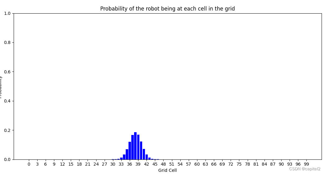
由图可见，通过观察模式，能够实现车辆的定位。