解读histogram_filter.py程序

（一）程序来自如下链接：

程序实现2D histogram_filter。

https://github.com/AtsushiSakai/PythonRobotics/blob/master/Localization/histogram_filter/histogram_filter.py

（二）参考文档：

(1)自动驾驶定位算法(九)-直方图滤波定位-腾讯云开发者社区-腾讯云

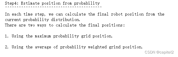
(2)histgoram_filter_localization_main.rst

（三）车辆运动轨迹

不考虑车辆位置概率的运动模式以及观察模式，仅根据运动方程得到的车辆运动轨迹，如下图示：

图1：车辆运动轨迹

程序中注释：

#grid_map = histogram_filter_localization(grid_map, u, z, yaw)

#draw_heat_map(grid_map.data, mx, my)

(四）根据车辆位置概率大小来预测车辆轨迹

根据histogram_filter_localization_main.rst描述，如何根据车辆位置的概率大小来预测车辆位置：

取车辆位置概率最大处作为车辆的预测轨迹，如下图示：

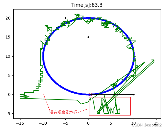
图2:车辆预测轨迹

从图2可以看出，刚开始车辆没有观察到地标的时候，其预测的位置轨迹与其实际的运行轨迹相差很大，说明车辆定位失败；而当车辆通过传感器观察到地标后，其预测位置逐渐与运行位置相接近，说明车辆定位成功。

（五）修改的程序代码

def main():
    print(__file__ + " start!!")

    # RF_ID positions [x, y]
    RF_ID = np.array([[10.0, 0.0],
                      [10.0, 10.0],
                      [0.0, 15.0],
                      [-5.0, 20.0]])

    time = 0.0

    xTrue = np.zeros((4, 1))
    px = []
    py = []
    px_est = []
    py_est = []
    px.append(xTrue[0, 0])
    py.append(xTrue[1, 0])
    #px_est.append(xTrue[0, 0])
    #py_est.append(xTrue[1, 0])

    grid_map = init_grid_map(XY_RESOLUTION, MIN_X, MIN_Y, MAX_X, MAX_Y)
    mx, my = calc_grid_index(grid_map)  # for grid map visualization

    while SIM_TIME >= time:
        time += DT
        print(f"{time=:.1f}")

        u = calc_control_input()

        yaw = xTrue[2, 0]  # Orientation is known
        xTrue, z, ud = observation(xTrue, u, RF_ID)
        px.append(xTrue[0, 0])
        py.append(xTrue[1, 0])


        grid_map = histogram_filter_localization(grid_map, u, z, yaw)
        r, c = np.where(grid_map.data == np.max(grid_map.data))
        px_est.append(r[0] * 0.5 - 15)
        py_est.append(c[0] * 0.5 - 5)

        if show_animation:
            plt.cla()
            # for stopping simulation with the esc key.
            plt.gcf().canvas.mpl_connect(
                'key_release_event',
                lambda event: [exit(0) if event.key == 'escape' else None])
            #draw_heat_map(grid_map.data, mx, my)
            plt.plot(xTrue[0, :], xTrue[1, :], "xr")
            plt.plot(RF_ID[:, 0], RF_ID[:, 1], ".k")
            plt.plot(px, py, ".b")
            plt.plot(px_est, py_est, linestyle = '-', color = 'g')

            for i in range(z.shape[0]):
                plt.plot([xTrue[0, 0], z[i, 1]],
                         [xTrue[1, 0], z[i, 2]],
                         "-k")
            plt.title("Time[s]:" + str(time)[0: 4])
            plt.pause(0.1)

    print("Done")