


一 实例描述
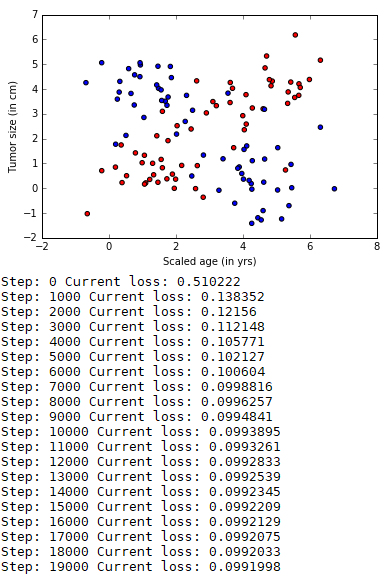
通过增加数据集的方式来改善过拟合情况,这里每次循环生成1000个数据。
二 代码
import tensorflow as tf
import numpy as np
import matplotlib.pyplot as plt
from sklearn.utils import shuffle
from matplotlib.colors import colorConverter, ListedColormap
# 对于上面的fit可以这么扩展变成动态的
from sklearn.preprocessing import OneHotEncoder
def onehot(y,start,end):
ohe = OneHotEncoder()
a = np.linspace(start,end-1,end-start)
b =np.reshape(a,[-1,1]).astype(np.int32)
ohe.fit(b)
c=ohe.transform(y).toarray()
return c
def generate(sample_size, num_classes, diff,regression=False):
np.random.seed(10)
mean = np.random.randn(2)
cov = np.eye(2)
#len(diff)
samples_per_class = int(sample_size/num_classes)
X0 = np.random.multivariate_normal(mean, cov, samples_per_class)
Y0 = np.zeros(samples_per_class)
for ci, d in enumerate(diff):
X1 = np.random.multivariate_normal(mean+d, cov, samples_per_class)
Y1 = (ci+1)*np.ones(samples_per_class)
X0 = np.concatenate((X0,X1))
Y0 = np.concatenate((Y0,Y1))
if regression==False: #one-hot 0 into the vector "1 0
Y0 = np.reshape(Y0,[-1,1])
#print(Y0.astype(np.int32))
Y0 = onehot(Y0.astype(np.int32),0,num_classes)
#print(Y0)
X, Y = shuffle(X0, Y0)
#print(X, Y)
return X,Y
# Ensure we always get the same amount of randomness
np.random.seed(10)
input_dim = 2
num_classes =4
X, Y = generate(120,num_classes, [[3.0,0],[3.0,3.0],[0,3.0]],True)
Y=Y%2
colors = ['r' if l == 0.0 else 'b' for l in Y[:]]
plt.scatter(X[:,0], X[:,1], c=colors)
plt.xlabel("Scaled age (in yrs)")
plt.ylabel("Tumor size (in cm)")
plt.show()
Y=np.reshape(Y,[-1,1])
learning_rate = 1e-4
n_input = 2
n_label = 1
n_hidden = 200
x = tf.placeholder(tf.float32, [None,n_input])
y = tf.placeholder(tf.float32, [None, n_label])
weights = {
'h1': tf.Variable(tf.truncated_normal([n_input, n_hidden], stddev=0.1)),
'h2': tf.Variable(tf.random_normal([n_hidden, n_label], stddev=0.1))
}
biases = {
'h1': tf.Variable(tf.zeros([n_hidden])),
'h2': tf.Variable(tf.zeros([n_label]))
}
layer_1 = tf.nn.relu(tf.add(tf.matmul(x, weights['h1']), biases['h1']))
#Leaky relus
layer2 =tf.add(tf.matmul(layer_1, weights['h2']),biases['h2'])
y_pred = tf.maximum(layer2,0.01*layer2)
reg = 0.01
loss=tf.reduce_mean((y_pred-y)**2)+tf.nn.l2_loss(weights['h1'])*reg+tf.nn.l2_loss(weights['h2'])*reg
train_step = tf.train.AdamOptimizer(learning_rate).minimize(loss)
#加载
sess = tf.InteractiveSession()
sess.run(tf.global_variables_initializer())
for i in range(20000):
X, Y = generate(1000,num_classes, [[3.0,0],[3.0,3.0],[0,3.0]],True)
Y=Y%2
Y=np.reshape(Y,[-1,1])
_, loss_val = sess.run([train_step, loss], feed_dict={x: X, y: Y})
if i % 1000 == 0:
print ("Step:", i, "Current loss:", loss_val)
colors = ['r' if l == 0.0 else 'b' for l in Y[:]]
plt.scatter(X[:,0], X[:,1], c=colors)
plt.xlabel("Scaled age (in yrs)")
plt.ylabel("Tumor size (in cm)")
nb_of_xs = 200
xs1 = np.linspace(-1, 8, num=nb_of_xs)
xs2 = np.linspace(-1, 8, num=nb_of_xs)
xx, yy = np.meshgrid(xs1, xs2) # create the grid
# Initialize and fill the classification plane
classification_plane = np.zeros((nb_of_xs, nb_of_xs))
for i in range(nb_of_xs):
for j in range(nb_of_xs):
#classification_plane[i,j] = nn_predict(xx[i,j], yy[i,j])
classification_plane[i,j] = sess.run(y_pred, feed_dict={x: [[ xx[i,j], yy[i,j] ]]} )
classification_plane[i,j] = int(classification_plane[i,j])
# Create a color map to show the classification colors of each grid point
cmap = ListedColormap([
colorConverter.to_rgba('r', alpha=0.30),
colorConverter.to_rgba('b', alpha=0.30)])
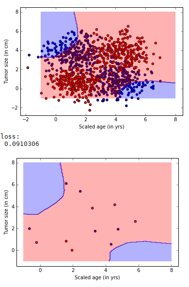
# Plot the classification plane with decision boundary and input samples
plt.contourf(xx, yy, classification_plane, cmap=cmap)
plt.show()
xTrain, yTrain = generate(12,num_classes, [[3.0,0],[3.0,3.0],[0,3.0]],True)
yTrain=yTrain%2
colors = ['r' if l == 0.0 else 'b' for l in yTrain[:]]
plt.scatter(xTrain[:,0], xTrain[:,1], c=colors)
plt.xlabel("Scaled age (in yrs)")
plt.ylabel("Tumor size (in cm)")
#plt.show()
yTrain=np.reshape(yTrain,[-1,1])
print ("loss:\n", sess.run(loss, feed_dict={x: xTrain, y: yTrain}))
nb_of_xs = 200
xs1 = np.linspace(-1, 8, num=nb_of_xs)
xs2 = np.linspace(-1, 8, num=nb_of_xs)
xx, yy = np.meshgrid(xs1, xs2) # create the grid
# Initialize and fill the classification plane
classification_plane = np.zeros((nb_of_xs, nb_of_xs))
for i in range(nb_of_xs):
for j in range(nb_of_xs):
#classification_plane[i,j] = nn_predict(xx[i,j], yy[i,j])
classification_plane[i,j] = sess.run(y_pred, feed_dict={x: [[ xx[i,j], yy[i,j] ]]} )
classification_plane[i,j] = int(classification_plane[i,j])
# Create a color map to show the classification colors of each grid point
cmap = ListedColormap([
colorConverter.to_rgba('r', alpha=0.30),
colorConverter.to_rgba('b', alpha=0.30)])
# Plot the classification plane with decision boundary and input samples
plt.contourf(xx, yy, classification_plane, cmap=cmap)
plt.show()
三 运行结果
四 说明
这次得到的模型测试值直接降到了0.9,比训练时还低。


 709
709

 被折叠的 条评论
为什么被折叠?
被折叠的 条评论
为什么被折叠?
 到【灌水乐园】发言


