基于matlab的传输函数特性分析

目录

1 概要

2. S域传输函数特性分析示例

3. pzmap(), pzplot() and zplane()

4. Z域传输函数特性分析示例

4.1 格型ＩＩＲ陷波滤波器例

4.2 离散传输函数表示：tf() vs filt()

4.3 zplane()生成的零极点图

4.4 freqz()和fvtool()

4.5 Tf2zp() vs tf2zpk()    

5. 小结

---

1 概要

       本文介绍基于matlab对给定传输函数进行特性分析的实验。

       连续系统通常用S域传输函数来表示，与之对应的则是离散系统通常用Z域传输函数来表示。

 

2. S域传输函数特性分析示例

      S域传输函数用于表示连续系统。  

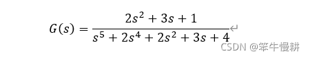
      问题：给定一个S域传输函数，试给出它的零极点和频域响应。 

 

clc;
clear all;
close all;
num = [2 3 1];
den = [1 2 0 2 3 4];
TRANF=tf(num,den)
[zeros poles gain]=tf2zp(num,den);
 
disp('Poles of transfer function are:');
disp(poles);
disp('Zeros of transfer function are:');
disp(zeros);
disp('Gain of transfer function are:');
disp(gain);

figure; pzmap(TRANF); title('pole-zero map by pzmap()');
figure; pzplot(TRANF); title('pole-zero map by pzplot()');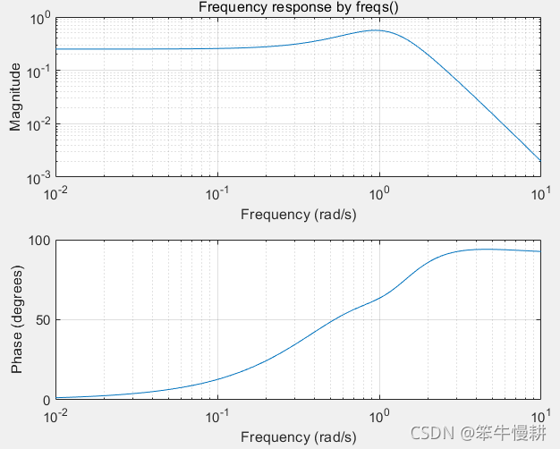
figure; freqs(num, den); title('Frequency response by freqs()');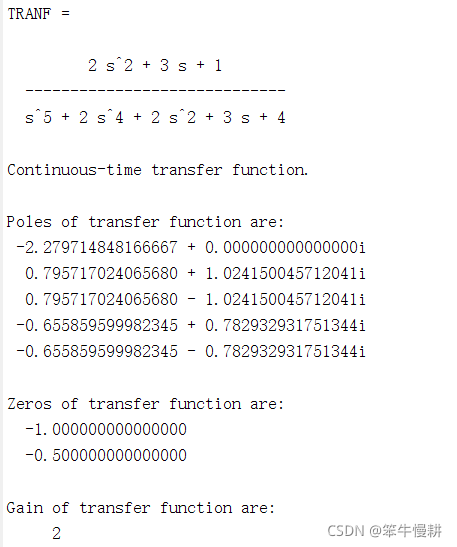

 

        tf()函数的功能：基于给定的分子(numerator)表达式和分母(denominator)表达式生成一个传输函数object，显示它的值的话会非常nice地显示出传输函数分式表示形式，非常直观。

        tf2zp()函数的功能: 基于给定的分子(numerator)表达式和分母(denominator)计算其零点、极点和直流增益。如上所示运行后会打印出零极点即直流增益结果。

        freqs()用于产生对应该传输函数的频域响应。

 

        pzmap()和pzplot()用于生成pole-zero图。在缺省条件下，两者生成的图相同。

 

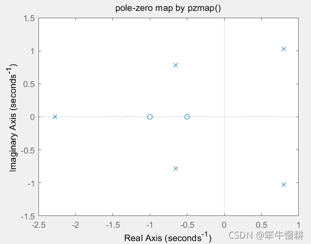
        但是pzmap()和pzplot()是有区别的。

3. pzmap(), pzplot() and zplane()

         pzmap and pzplot 都是Control System Toolbox中的函数，两者都既可以用于连续系统传输函数分析，也可以用于离散系统传输函数分析。区别在于pzplot可以返回一个handle to the plot object，基于这个handle用户可以进行更多的画图选项控制。It is explicit in the documentation of pzmap: "For additional options for customizing the appearance of the pole-zero plot,  use pzplot.".

        以下是一个利用pzplot的选项控制功能画图的示例。

% For demonstration of customization functionality of pzplot
Ts = 1;
HZ = tf(num, den, Ts, 'variable', 'z^-1');

figure;
pzplot(HZ); title('pole-zero map by pzplot() with customization');
h = findobj(gca, 'type', 'line');
set(h, 'markersize', 9)
text(real(roots(num)) - 0.1, imag(roots(num)) + 0.1, 'Zero')
text(real(roots(den)) - 0.1, imag(roots(den)) + 0.1, 'Pole')
axis equal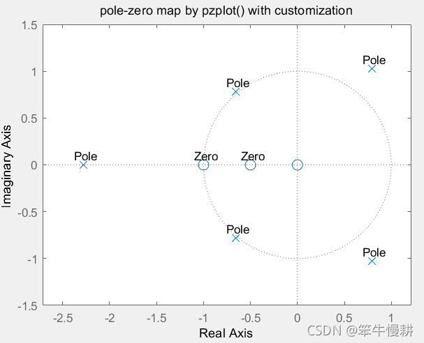

        这个图上的信息就比上面的缺省条件下生成的图要丰富得多。 

 

        此外，zplane()函数属于Signal Processing Toolbox，提供的功能与pzmap()和pzplot()相似，但是使用语法不一样。而且zplane只能用于discrete系统传输函数的分析。后面离散系统的分析我们会用到zplane().

 

[1] https://www.mathworks.com/matlabcentral/answers/509011-pzmap-vs-pzplot-vs-zplane

[2] MATLAB: What is the difference between pzmap and pzplot? - Stack Overflow

 

4. Z域传输函数特性分析示例

        离散系统的传输函数用Z域传输函数表示。

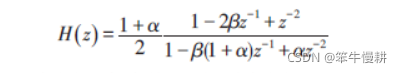
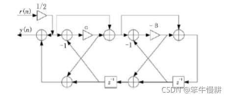
4.1 格型ＩＩＲ陷波滤波器例

        以下是一个格型IIR陷波滤波器的特性分析示例。其传输函数和结构图如下所示：

 

% Discrete system zero-pole analysis
alpha = 0.9962;
beta  = 0.8763;
num = ((1+alpha)/2)*[1 -2*beta 1]
den = [1 -beta*(1+alpha) alpha]
ZtranF = tf(num,den,1)
ZtranF1 = filt(num,den,1)
[zeros poles gain]=tf2zp(num,den);
[zeros1 poles1 gain1]=tf2zpk(num,den); % What is the difference between tf2zp and tf2zpk

disp('Poles of transfer function are:');
disp(poles);
disp('Zeros of transfer function are:');
disp(zeros);
disp('Gain of transfer function are:');
disp(gain);
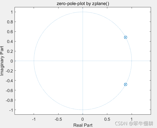
figure; zplane(num,den); title('zero-pole-plot by zplane()'); % zplane() For discrete system.

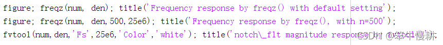
figure; freqz(num, den); title('Frequency response by freqz() with default setting');
figure; freqz(num, den,500,25e6); title('Frequency response by freqz(), with n=500');
fvtool(num,den,'Fs',25e6,'Color','white'); title('notch\_flt magnitude response by fvtool()');

figure; impz(num,den);  title('Impulse response by freqz()');

4.2 离散传输函数表示：tf() vs filt()

        从结果来看，tf()和filt()有微妙差别，如下图所示：

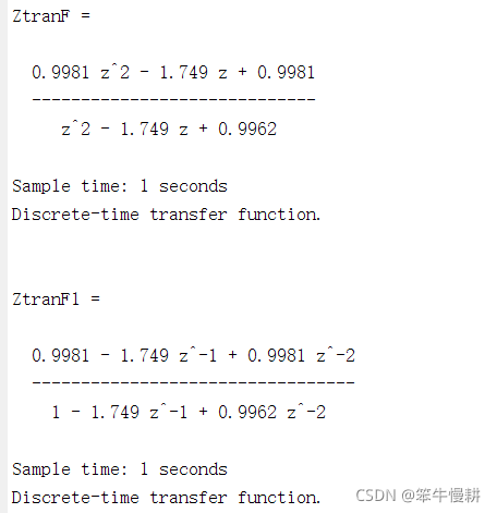
         首先，需要注意的是，tf()必须将Ts设置为某个正值才表示是分析离散的Z域传输函数。tf生成的传输函数与连续系统的传输函数的表示习惯相同，用z的正指数表示，而filt()生成的则是离散系统的表示习惯，用z的负指数项表示。没有本质区别，但是可能用的filt()更好吧。

4.3 zplane()生成的零极点图

        如前所述，离散系统的零极点图可以用zplane()生成。但是也同样可以pzmap()和pzplot()生成，表示效果略有差异。

4.4 freqz()和fvtool()

        freqz()和fvtool()都可以用来生成频域响应。

        但是以下三条语句却产生了不同的结果。

 

 

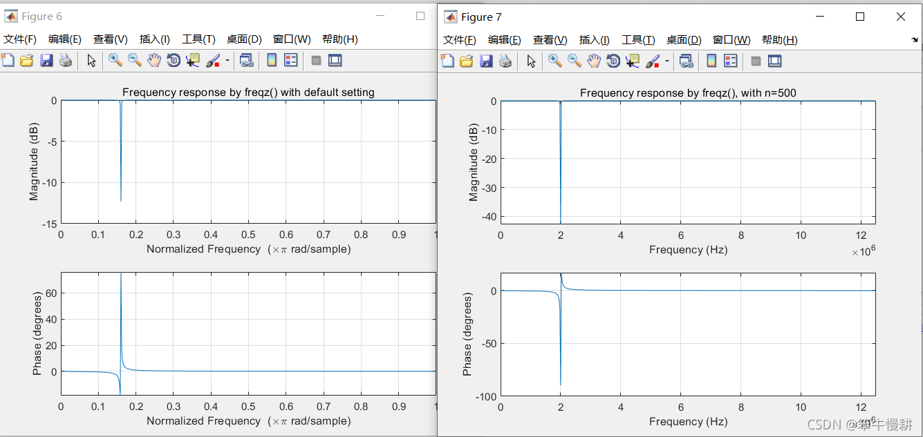
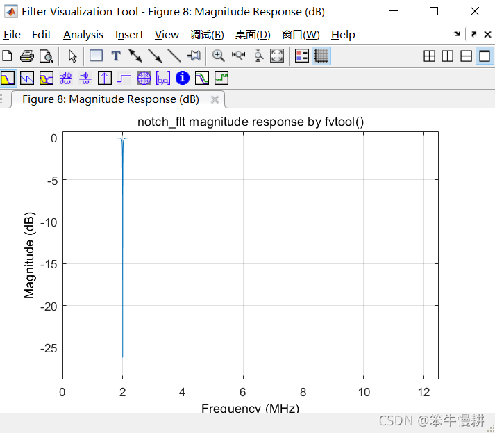
        很显然，3张图中所显示的陷波频点的衰减各不相同。可能是设置不同所导致的差别，有待进一步调查分析。

 

4.5 Tf2zp() vs tf2zpk()    

tf2zp (Signal Processing Toolbox) (northwestern.edu)

Note You should use tf2zp when working with positive powers (s2 + s + 1), such as in continuous-time transfer functions. A similar function, tf2zpk, is more useful when working with transfer functions expressed in inverse powers (1 + z-1 + z-2), which is how transfer functions are usually expressed in DSP.

 

tf2zpk (Signal Processing Toolbox) (northwestern.edu)

Note You should use tf2zpk when working with transfer functions expressed in inverse powers (1 + z-1 + z-2), which is how transfer functions are usually expressed in DSP. A similar function, tf2zp, is more useful for working with positive powers (s2 + s + 1), such as in continuous-time transfer functions.

 

另外几个相关的函数：sos2zp, ss2zp, tf2sos, tf2ss, tf2zp, zp2tf

 

5. 小结

        仓促而就。Ｍａｔｌａｂ提供了非常丰富的传输函数相关的函数和工具，值得慢慢挖掘。当然ｐｙｔｈｏｎ中ｓｃｉｐｙ库也有相对应的函数工具库，以后有时间再来学习整理。