Excel中的VLOOKUP，第2部分：在没有数据库的情况下使用VLOOKUP

最新推荐文章于 2022-07-13 16:31:16 发布

culinxia2707

最新推荐文章于 2022-07-13 16:31:16 发布

阅读量834

点赞数

文章标签：数据库 python java 人工智能机器学习

原文链接：https://www.howtogeek.com/howto/14455/vlookup-in-excel-part-2-using-vlookup-without-a-database/

版权

In a recent article, we introduced the Excel function called VLOOKUP and explained how it could be used to retrieve information from a database into a cell in a local worksheet. In that article we mentioned that there were two uses for VLOOKUP, and only one of them dealt with querying databases. In this article, the second and final in the VLOOKUP series, we examine this other, lesser known use for the VLOOKUP function.

在最近的文章中，我们介绍了称为VLOOKUP的Excel函数，并解释了如何使用该函数将数据库中的信息检索到本地工作表中的单元格中。在那篇文章中，我们提到了VLOOKUP有两种用法，其中只有一种用于查询数据库。在本文(VLOOKUP系列的第二篇也是最后一篇)中，我们研究了VLOOKUP函数的另一种鲜为人知的用法。

If you haven’t already done so, please read the first VLOOKUP article – this article will assume that many of the concepts explained in that article are already known to the reader.

如果您尚未这样做，请阅读第一篇VLOOKUP文章 -本文将假定读者已经知道该文章中解释的许多概念。

When working with databases, VLOOKUP is passed a “unique identifier” that serves to identify which data record we wish to find in the database (e.g. a product code or customer ID). This unique identifier must exist in the database, otherwise VLOOKUP returns us an error. In this article, we will examine a way of using VLOOKUP where the identifier doesn’t need to exist in the database at all. It’s almost as if VLOOKUP can adopt a “near enough is good enough” approach to returning the data we’re looking for. In certain circumstances, this is exactly what we need.

使用数据库时，VLOOKUP传递了一个“唯一标识符”，该标识符用于标识我们希望在数据库中找到的数据记录(例如产品代码或客户ID)。该唯一标识符必须存在于数据库中，否则VLOOKUP向我们返回错误。在本文中，我们将研究一种使用VLOOKUP的方法，其中标识符根本不需要在数据库中存在。 VLOOKUP几乎可以采用“足够近就足够好”的方法来返回我们正在寻找的数据。在某些情况下，这正是我们所需要的。

We will illustrate this article with a real-world example – that of calculating the commissions that are generated on a set of sales figures. We will start with a very simple scenario, and then progressively make it more complex, until the only rational solution to the problem is to use VLOOKUP. The initial scenario in our fictitious company works like this: If a salesperson creates more than $30,000 worth of sales in a given year, the commission they earn on those sales is 30%. Otherwise their commission is only 20%. So far this is a pretty simple worksheet:

我们将以一个真实的例子来说明这篇文章-计算一组销售数据所产生的佣金。我们将从一个非常简单的场景开始，然后逐步使其变得更加复杂，直到对该问题唯一的合理解决方案是使用VLOOKUP。我们在虚拟公司中的初始方案是这样的：如果销售人员在给定年份创造了价值30,000美元以上的销售，则他们从这些销售中获得的佣金为30％。否则，他们的佣金仅为20％。到目前为止，这是一个非常简单的工作表：

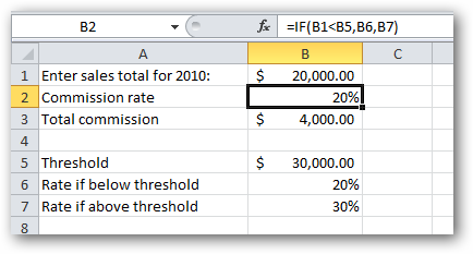
To use this worksheet, the salesperson enters their sales figures in cell B1, and the formula in cell B2 calculates the correct commission rate they are entitled to receive, which is used in cell B3 to calculate the total commission that the salesperson is owed (which is a simple multiplication of B1 and B2).

要使用此工作表，销售人员在单元格B1中输入他们的销售数字，单元格B2中的公式将计算出他们有权获得的正确佣金率，并在单元格B3中使用该佣金率来计算应支付给销售人员的总佣金(是B1和B2的简单乘法)。

The cell B2 contains the only interesting part of this worksheet – the formula for deciding which commission rate to use: the one below the threshold of $30,000, or the one above the threshold. This formula makes use of the Excel function called IF. For those readers that are not familiar with IF, it works like this:

单元格B2包含此工作表中唯一有趣的部分–确定使用哪种佣金率的公式：低于 $ 30,000阈值的阈值或高于 $ 30,000阈值的阈值。该公式利用了称为IF的Excel函数。对于那些不熟悉IF的读者，它的工作方式如下：

IF(condition,value if true,value if false)

IF( 条件，如果为true，则为false )

Where the condition is an expression that evaluates to either true or false. In the example above, the condition is the expression B1<B5, which can be read as “Is B1 less than B5?”, or, put another way, “Are the total sales less than the threshold”. If the answer to this question is “yes” (true), then we use the value if true parameter of the function, namely B6 in this case – the commission rate if the sales total was below the threshold. If the answer to the question is “no” (false), then we use the value if false parameter of the function, namely B7 in this case – the commission rate if the sales total was above the threshold.

条件是表达式，其结果为true或false 。在上面的示例中，条件是表达式B1 <B5 ，可以理解为“ B1是否小于B5？”，或者换句话说，“总销售额是否小于阈值”。如果对这个问题的回答是“是”(true)，则我们使用该函数的参数if true的值，在这种情况下为B6 –如果销售总额低于阈值，则为佣金率。如果问题的答案为“否”(否)，那么我们使用该函数的false参数值(在这种情况下为B7) –如果销售总额高于阈值，则为佣金率。

As you can see, using a sales total of $20,000 gives us a commission rate of 20% in cell B2. If we enter a value of $40,000, we get a different commission rate:

如您所见，使用总计20,000美元的销售额，我们在单元格B2中的佣金率为20％。如果我们输入的值为$ 40,000，我们将获得不同的佣金率：

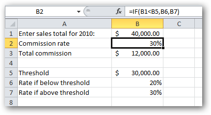
So our spreadsheet is working.

因此，我们的电子表格正在运行。

Let’s make it more complex. Let’s introduce a second threshold: If the salesperson earns more than $40,000, then their commission rate increases to 40%:

让我们使其更复杂。让我们介绍第二个阈值：如果销售人员的收入超过40,000美元，那么他们的佣金率将提高到40％：

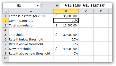
Easy enough to understand in the real world, but in cell B2 our formula is getting more complex. If you look closely at the formula, you’ll see that the third parameter of the original IF function (the value if false) is now an entire IF function in its own right. This is called a nested function (a function within a function). It’s perfectly valid in Excel (it even works!), but it’s harder to read and understand.

在现实世界中很容易理解，但是在单元格B2中，我们的公式变得越来越复杂。如果仔细看一下公式，您会发现原始IF函数的第三个参数( 如果为false的值 )现在本身就是整个IF函数。这称为嵌套函数 (函数中的函数)。它在Excel中是完全有效的(甚至可以使用！)，但是很难阅读和理解。

We’re not going to go into the nuts and bolts of how and why this works, nor will we examine the nuances of nested functions. This is a tutorial on VLOOKUP, not on Excel in general.

我们不会深入探讨其工作方式和原因，也不会研究嵌套函数的细微差别。这是有关VLOOKUP的教程，通常不是有关Excel的教程。

Anyway, it gets worse! What about when we decide that if they earn more than $50,000 then they’re entitled to 50% commission, and if they earn more than $60,000 then they’re entitled to 60% commission?

无论如何，情况变得更糟！当我们决定如果他们的收入超过50,000美元，那么他们有权获得50％的佣金；如果他们的收入超过60,000美元，那么他们有权获得60％的佣金，那该怎么办？

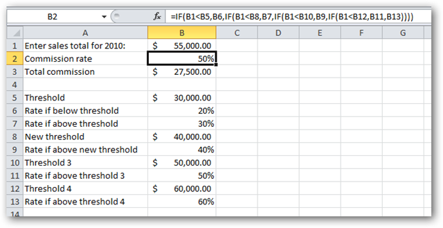
Now the formula in cell B2, while correct, has become virtually unreadable. No-one should have to write formulae where the functions are nested four levels deep! Surely there must be a simpler way?

现在，单元格B2中的公式虽然正确，但实际上已变得不可读。没有人应该写公式来将函数嵌套四个层次！当然必须有一种更简单的方法吗？

There certainly is. VLOOKUP to the rescue!

当然有。 VLOOKUP进行救援！

Let’s redesign the worksheet a bit. We’ll keep all the same figures, but organize it in a new way, a more tabular way:

让我们重新设计工作表。我们将保留所有相同的数字，但以一种新的方式，以一种更表格的方式来组织它：

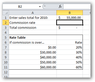
Take a moment and verify for yourself that the new Rate Table works exactly the same as the series of thresholds above.

请花点时间为自己核实新的费率表与上述一系列阈值完全相同。

Conceptually, what we’re about to do is use VLOOKUP to look up the salesperson’s sales total (from B1) in the rate table and return to us the corresponding commission rate. Note that the salesperson may have indeed created sales that are not one of the five values in the rate table ($0, $30,000, $40,000, $50,000 or $60,000). They may have created sales of $34,988. It’s important to note that $34,988 does not appear in the rate table. Let’s see if VLOOKUP can solve our problem anyway…

从概念上讲，我们要做的是使用VLOOKUP在费率表中查找销售员的销售总额(来自B1)，并向我们返回相应的佣金率。请注意，销售人员可能确实创建了不是费率表中的五个值之一的销售($ 0，$ 30,000，$ 40,000，$ 50,000或$ 60,000)。他们可能创造了$ 34,988的销售额。请注意，费率表中未显示$ 34,988。让我们看看VLOOKUP是否可以解决我们的问题……

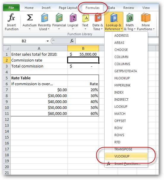
We select cell B2 (the location we want to put our formula), and then insert the VLOOKUP function from the Formulas tab:

我们选择单元格B2(要放置公式的位置)，然后从“ 公式”选项卡中插入VLOOKUP函数：

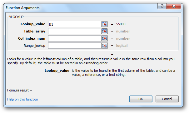
The Function Arguments box for VLOOKUP appears. We fill in the arguments (parameters) one by one, starting with the Lookup_value, which is, in this case, the sales total from cell B1. We place the cursor in the Lookup_value field and then click once on cell B1:

出现VLOOKUP的功能参数框。我们从Lookup_value开始一个接一个地填充参数(参数)，在这种情况下，它是来自单元格B1的销售总额。我们将光标放在Lookup_value字段中，然后在单元格B1上单击一次：

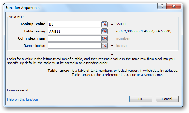
Next we need to specify to VLOOKUP what table to lookup this data in. In this example, it’s the rate table, of course. We place the cursor in the Table_array field, and then highlight the entire rate table – excluding the headings:

接下来，我们需要向VLOOKUP指定在哪个表中查找此数据。当然，在此示例中，这是费率表。我们将光标放在Table_array字段中，然后突出显示整个汇率表- 不包括标题 ：

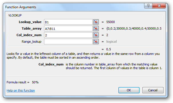
Next we must specify which column in the table contains the information we want our formula to return to us. In this case we want the commission rate, which is found in the second column in the table, so we therefore enter a 2 into the Col_index_num field:

接下来，我们必须指定表中的哪一列包含我们希望公式返回给我们的信息。在这种情况下，我们需要在表的第二列中找到的佣金率，因此，我们在Col_index_num字段中输入2 ：

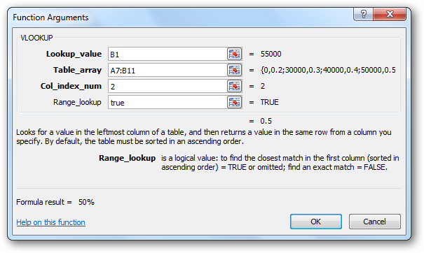
Finally we enter a value in the Range_lookup field.

最后，我们在Range_lookup字段中输入一个值。

Important: It is the use of this field that differentiates the two ways of using VLOOKUP. To use VLOOKUP with a database, this final parameter, Range_lookup, must always be set to FALSE, but with this other use of VLOOKUP, we must either leave it blank or enter a value of TRUE. When using VLOOKUP, it is vital that you make the correct choice for this final parameter.

要点：使用此字段可以区分使用VLOOKUP的两种方式。 要将VLOOKUP与数据库一起使用，必须始终将此最终参数Range_lookup设置为FALSE ，但在其他使用VLOOKUP的情况下，我们必须将其保留为空白或输入TRUE 。 使用VLOOKUP时，至关重要的是您要为该最终参数做出正确的选择。

To be explicit, we will enter a value of true in the Range_lookup field. It would also be fine to leave it blank, as this is the default value:

明确地说，我们将在Range_lookup字段中输入true值。也可以将其保留为空白，因为这是默认值：

We have completed all the parameters. We now click the OK button, and Excel builds our VLOOKUP formula for us:

我们已经完成了所有参数。现在，我们单击“ 确定”按钮，Excel将为我们建立VLOOKUP公式：

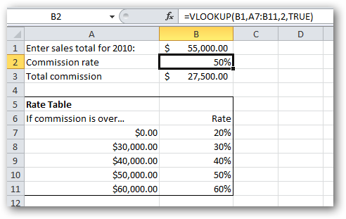
If we experiment with a few different sales total amounts, we can satisfy ourselves that the formula is working.

如果我们尝试一些不同的销售总额，我们可以使自己满意该公式在起作用。

Conclusion

结论

In the “database” version of VLOOKUP, where the Range_lookup parameter is FALSE, the value passed in the first parameter (Lookup_value) must be present in the database. In other words, we’re looking for an exact match.

在VLOOKUP的“数据库”版本中， Range_lookup参数为FALSE ，第一个参数( Lookup_value )中传递的值必须存在于数据库中。换句话说，我们正在寻找完全匹配的内容。

But in this other use of VLOOKUP, we are not necessarily looking for an exact match. In this case, “near enough is good enough”. But what do we mean by “near enough”? Let’s use an example: When searching for a commission rate on a sales total of $34,988, our VLOOKUP formula will return us a value of 30%, which is the correct answer. Why did it choose the row in the table containing 30% ? What, in fact, does “near enough” mean in this case? Let’s be precise:

但是，在VLOOKUP的这种其他用法中，我们不一定要寻找完全匹配的内容。在这种情况下，“足够近就足够好”。但是，“足够接近”是什么意思？让我们举一个例子：当搜索销售总额为34,988美元的佣金率时，我们的VLOOKUP公式将为我们返回30％的值，这是正确的答案。为什么选择表中包含30％的行？实际上，在这种情况下，“足够接近”意味着什么？确切地说：

When Range_lookup is set to TRUE (or omitted), VLOOKUP will look in column 1 and match the highest value that is not greater than the Lookup_value parameter.

当Range_lookup设置为TRUE (或省略)时，VLOOKUP将在列1中查找并匹配不大于 Lookup_value参数的最大值 。