如何使用VLOOKUP在Google表格中查找数据

VLOOKUP is one of the most misunderstood functions in Google Sheets. It allows you to search through and link together two sets of data in your spreadsheet with a single search value. Here’s how to use it.

VLOOKUP是Google表格中最容易被误解的功能之一。 它使您可以使用单个搜索值搜索电子表格中的两组数据并将其链接在一起。 这是使用方法。

Unlike Microsoft Excel, there’s no VLOOKUP wizard to help you in Google Sheets, so you have to type the formula manually.

与Microsoft Excel不同，没有VLOOKUP向导可以在Google表格中为您提供帮助，因此您必须手动输入公式。

VLOOKUP在Google表格中的工作方式 (How VLOOKUP Works in Google Sheets)

VLOOKUP might sound confusing, but it’s pretty simple once you understand how it works.  A formula that uses the VLOOKUP function has four arguments.

VLOOKUP听起来可能令人困惑，但是一旦您了解了它的工作原理，它就非常简单。 使用VLOOKUP函数的公式具有四个参数。

The first is the search key value you’re looking for, and the second is the cell range you’re searching (e.g., A1 to D10). The third argument is the column index number from your range to be searched, where the first column in your range is number 1, the next is number 2, and so on.

第一个是您要搜索的搜索键值，第二个是您要搜索的单元格范围(例如，A1至D10)。 第三个参数是要搜索的范围中的列索引号，范围中的第一列是数字1，下一个是数字2，依此类推。

The fourth argument is whether the search column has been sorted or not.

第四个参数是搜索列是否已排序。

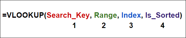
The final argument is only important if you’re looking for the closest match to your search key value. If you’d rather return exact matches to your search key, you set this argument to FALSE.

仅当您正在