excel vlookup_Excel VLOOKUP公式错误之谜

最新推荐文章于 2022-09-10 16:14:33 发布

culiao2169

最新推荐文章于 2022-09-10 16:14:33 发布

阅读量869

点赞数

文章标签：字符串 python java excel 正则表达式

原文链接：https://contexturesblog.com/archives/2018/02/15/excel-vlookup-formula-error-mystery/

版权

excel vlookup

Someone sent me a workbook in which a simple VLOOKUP formula was returning #N/A errors, instead of the correct results. The product numbers looked the same, but Excel didn't match them in the lookup. Can you solve this VLOOKUP formula error mystery?

有人给我寄了一个工作簿，其中一个简单的VLOOKUP公式返回了＃N / A错误，而不是正确的结果。产品编号看起来相同，但是Excel在查找中不匹配它们。您能解决这个VLOOKUP公式错误的奥秘吗？

VLOOKUP公式错误 (VLOOKUP Formula Error)

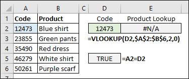
To show you the problem, here's a screenshot of the lookup table, and the VLOOKUP formula. The formula in cell D5 says that the blue cell (A2) and the green cell (D2) are equal.

为了向您展示问题，这是查找表和VLOOKUP公式的屏幕截图。单元格D5中的公式表示蓝色单元格(A2)和绿色单元格(D2)相等。

However, there's a VLOOKUP formula error in cell E2. Instead of returning the product name, "Blue shirt", the result is #N/A.

但是，单元格E2中存在VLOOKUP公式错误。结果没有返回产品名称“蓝色衬衫”，而是返回＃N / A。

获取VLOOKUP示例文件 (Get the VLOOKUP Sample File)

If you love an Excel challenge, click here to download the sample file, and see if you can fix the problem - it's a tricky one!

如果您喜欢Excel挑战，请单击此处下载示例文件，然后查看是否可以解决问题-这是一个棘手的问题！

If you're not sure where to start looking for the problem, there are VLOOKUP troubleshooting tips on my site.
如果不确定从哪里开始寻找问题，我的网站上有VLOOKUP故障排除提示。
The sample file also has a sheet that shows my troubleshooting steps, and another sheet shows my formula that fixes the problem.
该示例文件还具有一张显示我的疑难解答步骤的表格，另一张显示了解决该问题的公式。

WARNING – The troubleshooting steps for the VLOOKUP formula mystery start in the next section.

警告 –有关VLOOKUP公式奥秘的疑难解答步骤将从下一部分开始。

Stop reading here, if you don't want to see how I fixed the VLOOKUP formula error.

如果您不想了解如何解决VLOOKUP公式错误，请在这里停止阅读。

。

VLOOKUP故障排除第1部分 (VLOOKUP Troubleshooting Part 1)

Usually, this type of VLOOKUP error occurs when one value is a real number, and the other is text number. See the details for that type of Number/Text problem on my website.

通常，当一个值是实数而另一个是文本数时，会发生这种VLOOKUP错误。在我的网站上查看有关该类型的数字/文本问题的详细信息。

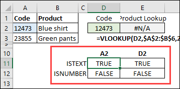
To test the numbers in the sample file, I used the ISTEXT and ISNUMBER functions. The screen show below shows the results of that test, for the values in A2 and D2.

为了测试示例文件中的数字，我使用了ISTEXT和ISNUMBER函数。下面的屏幕显示了A2和D2中的值的测试结果。

Both cells contain text, not real numbers, so a Number/Text issue isn't causing the errors in this workbook.

两个单元格都包含文本，而不是实数，因此“数字/文本”问题不会引起此工作簿中的错误。

VLOOKUP故障排除第2部分 (VLOOKUP Troubleshooting Part 2)

Another common cause for VLOOKUP errors is extra characters in one of the cells – usually extra space characters.

VLOOKUP错误的另一个常见原因是其中一个单元格中的多余字符，通常是多余的空格字符。

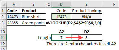
Using the LEN function, I checked the length of the string in each cell.

使用LEN函数，我检查了每个单元格中字符串的长度。

There are 7 characters in A2, and only 5 characters in cell D2

A2中有7个字符，而单元格D2中只有5个字符

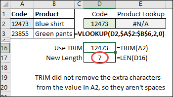
The TRIM function will remove leading, trailing, and duplicate spaces.

TRIM函数将删除前导，尾随和重复的空格。

In cell D16, I used TRIM on the value in A2.
在单元格D16中，我对A2中的值使用了TRIM。
Then, I checked the length of the trimmed string.
然后，我检查了修剪后的琴弦的长度。

There was no change, so the extra characters are NOT normal space characters.

没有变化，因此多余的字符不是普通的空格字符。

VLOOKUP故障排除第3部分 (VLOOKUP Troubleshooting Part 3)

The next step is to figure out what those extra characters are.

下一步是弄清楚那些多余的字符是什么。

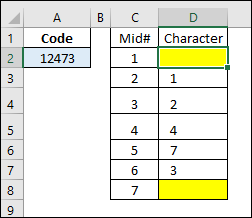
We know there are 7 characters in cell A2, so I listed the numbers 1-7 on a worksheet.
我们知道单元格A2中有7个字符，因此我在工作表上列出了数字1-7。
In the next column, the MID function extracts one character at each position.
在下一列中，MID函数在每个位置提取一个字符。

The numbers from cell A2 appear in positions 2-6, and there are hidden characters at the start and end of the string.

单元格A2中的数字出现在位置2-6，并且在字符串的开头和结尾处都有隐藏的字符。

In the next column, I used the CODE function, to see what each character number is. Some characters, such as non-printing characters 0-30, can be removed with the CLEAN function. Let's see if our hidden characters are one of those.

在下一列中，我使用CODE函数来查看每个字符数是什么。可以使用CLEAN功能删除某些字符，例如非打印字符0-30。让我们看看我们的隐藏字符是否是其中之一。

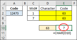
No, Excel says that cells D2 and D8 contain character #63.

不，Excel表示单元格D2和D8包含字符＃63。

There isn't a non-printing character with code 63 though, so what is happening?

但是，代码中没有非打印字符63，这是怎么回事？

I typed 63 in cell D10, and used the CHAR function to see the character with that code number. Hmmm…it's a question mark.

我在单元格D10中键入63，并使用CHAR函数查看具有该代码号的字符。嗯...这是一个问号。

So those hidden characters are not really questions marks, but Excel is confused, and returns that code number anyway. (I found that clue on the Mr. Excel forum).

因此，那些隐藏的字符并不是真正的问号，但是Excel感到困惑，并且无论如何都会返回该代码号。 (我在Excel先生论坛上找到了线索 )。

CODE and CHAR use the basic ANSI character set in Windows, which has a maximum code number of 255.
CODE和CHAR使用Windows中的基本ANSI字符集，最大字符数为255。
The hidden characters are probably from a different character set, and have a code number greater than 255
隐藏的字符可能来自不同的字符集，并且其代码号大于255

Whatever they are, we can't use CLEAN to remove those hidden characters.

无论它们是什么，我们都不能使用CLEAN删除那些隐藏的字符。

VLOOKUP故障排除第4部分 (VLOOKUP Troubleshooting Part 4)

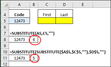
To fix the formula, we don't need to know what those hidden characters are. However, I was curious to find out if they were both the same character, or two different characters.

要确定公式，我们不需要知道那些隐藏字符是什么。但是，我很想知道它们是相同的字符还是两个不同的字符。

To test that, I used SUBSTITUTE, to replace any instances of the first hidden character, with an empty string. That reduces the string by 1 character
为了测试这一点，我使用SUBSTITUTE将一个第一个隐藏字符的任何实例替换为一个空字符串。这样可以将字符串减少1个字符
When I used SUBSTITUTE for each of the characters, both hidden characters were removed from the string.
当我对每个字符使用SUBSTITUTE时，两个隐藏的字符都从字符串中删除了。

If you really need to identify one of these strange characters, use the AscW function in a macro, or in the Immediate Window. This bit of code will show the character number for the first character in the active cell.

如果您确实需要识别这些奇怪的字符之一，请在宏或“即时窗口”中使用AscW函数。此代码位将显示活动单元格中第一个字符的字符号。

Sub GetCode()
  Debug.Print AscW(ActiveCell.Value)
End Sub

With that code, I learned that the hidden characters in this file are characters 8237 (cell C5) and 8236 (cell D5)

通过该代码，我了解到此文件中的隐藏字符是字符8237(单元格C5)和8236(单元格D5)

VLOOKUP公式错误的解决方案 (Solution to VLOOKUP Formula Error)

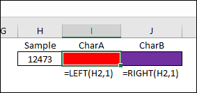
To fix the problem, I set up a "hidden character extraction range".

为了解决该问题，我设置了“隐藏字符提取范围”。

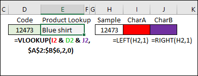
In cell H2, a sample code was pasted from the lookup table
在单元格H2中，从查找表粘贴了示例代码
In cell I2, a LEFT formula pulls out the first character: =LEFT(H2,1)
在单元格I2中，LEFT公式提取第一个字符：= LEFT(H2,1)
In cell J2, a RIGHT formula pulls out the last character: =RIGHT(H2,1)
在单元格J2中，RIGHT公式提取出最后一个字符：= RIGHT(H2,1)

NOTE: You could put this information on a hidden sheet. I left them on the same sheet as the VLOOKUP, so it's easier to see how they're used.

注意：您可以将此信息放在隐藏的工作表上。我将它们与VLOOKUP放在同一张纸上，因此更容易看到它们的用法。

Then, combine those hidden characters with the product number in the VLOOKUP formula in cell E2, to get the product name: =VLOOKUP(I2 & D2 & J2, $A$2:$B$6,2,0)

然后，将这些隐藏的字符与单元格E2中VLOOKUP公式中的产品编号组合，以得到产品名称：= VLOOKUP( I2＆D2＆J2 ，$ A $ 2：$ B $ 6,2,0)