


目录
alexnet论文翻译链接:ImageNet Classification with Deep Convolutional Neural Networks(AlexNet论文翻译(附原文))_机器学习我不学习的博客-CSDN博客
1.网络结构
AlexNet网络结构如下图所示:

图中分为上下两部分,分别是在两块GPU上进行训练,因此上下部分结构是相同的,可以只看下边部分。该神经网络有五个卷积层,其中有些卷积层后还会连接个最大池化层,三个全连接层,还有排在最后的1000路的softmax层组成,其产生一个覆盖1000类标签的分布。
第二、第四和第五个卷积层的核只连接到前一个卷积层也位于同一GPU中的那些核映射上。第三个卷积层的核被连接到第二个卷积层中的所有核映射上。全连接层中的神经元被连接到前一层中所有的神经元上。响应归一化层跟在第一、第二个卷积层后面。
该网络的亮点在于:
(1)首次利用GPU进行网络加速训练。
(2)使用了ReLU激活函数,而不是传统的Sigmoid激活函数以及Tanh激活函数。(smoid求导比较麻烦而且当网路比较深的时候会出现梯度消失)
(3)使用了LRN局部响应归一化。
(4)在全连接层的前两层中使用了Dropout随机失活神经元操作,以减少过拟合。
2.激活函数
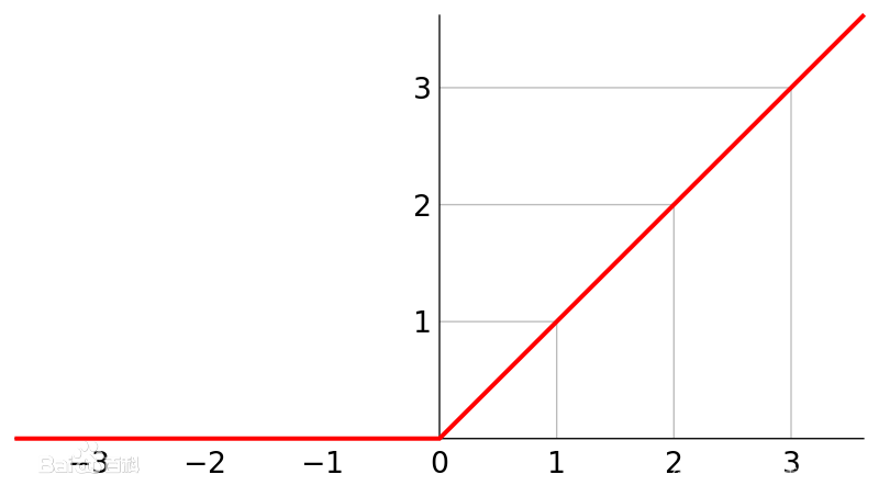
本文采用的激活函数为ReLu函数。
在神经网络中,激活函数负责将来自节点的加权输入转换为该输入的节点或输出的激活。一个神经网络由层节点组成,并学习将输入的样本映射到输出。对于给定的节点,将输入乘以节点中的权重,并将其相加。此值称为节点的summed activation。然后,经过求和的激活通过一个激活函数转换并定义特定的输出或节点的“activation”。
最简单的激活函数被称为线性激活,其中根本没有应用任何转换。 一个仅由线性激活函数组成的网络很容易训练,但不能学习复杂的映射函数。线性激活函数仍然用于预测一个数量的网络的输出层(例如回归问题)。
非线性激活函数是更好的,因为它们允许节点在数据中学习更复杂的结构 。两个广泛使用的非线性激活函数是sigmoid 函数和双曲正切 激活函数。
Sigmoid 激活函数 ,也被称为 Logistic函数神经网络,传统上是一个非常受欢迎的神经网络激活函数。函数的输入被转换成介于0.0和1.0之间的值。大于1.0的输入被转换为值1.0,同样,小于0.0的值被折断为0.0。所有可能的输入函数的形状都是从0到0.5到1.0的 s 形。在很长一段时间里,直到20世纪90年代早期,这是神经网络的默认激活方式。
双曲正切函数 ,简称 tanh,是一个形状类似的非线性激活函数,输出值介于-1.0和1.0之间。在20世纪90年代后期和21世纪初期,由于使用 tanh 函数的模型更容易训练,而且往往具有更好的预测性能,因此 tanh 函数比 Sigmoid激活函数更受青睐。
Sigmoid和 tanh 函数的一个普遍问题是它们值域饱和了 。这意味着,大值突然变为1.0,小值突然变为 -1或0。此外,函数只对其输入中间点周围的变化非常敏感。无论作为输入的节点所提供的求和激活是否包含有用信息,函数的灵敏度和饱和度都是有限的。一旦达到饱和状态,学习算法就需要不断调整权值以提高模型的性能。
最后,随着硬件能力的提高,通过 gpu 的非常深的神经网络使用Sigmoid 和 tanh 激活函数不容易训练。在大型网络深层使用这些非线性激活函数不能接收有用的梯度信息。错误通过网络传播回来,并用于更新权重。每增加一层,错误数量就会大大减少。这就是所谓的消失梯度 问题,它能有效地阻止深层(多层)网络的学习。
为了训练深层神经网络,需要一个激活函数神经网络,它看起来和行为都像一个线性函数,但实际上是一个非线性函数,允许学习数据中的复杂关系 。该函数还必须提供更灵敏的激活和输入,避免饱和。因此,ReLU出现了,采用 ReLU 可以是深度学习革命中为数不多的里程碑之一 。ReLU 是一个分段线性函数,如果输入大于0,直接返回作为输入提供的值;如果输入是0或更小,返回值0。
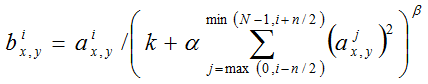
3.LRN局部响应归一化
局部响应归一化原理是仿造生物学上活跃的神经元对相邻神经元的抑制现象(侧抑制),对局部神经元的活动创建竞争机制,使得其中响应比较大的值变得相对更大,并抑制其他反馈较小的神经元,增强了模型的泛化能力。LRN通过在相邻卷积核生成的feature map之间引入竞争,从而有些本来在feature map中显著的特征在A中更显著,而在相邻的其他feature map中被抑制,这样让不同卷积核产生的feature map之间的相关性变小。
4. Dropout(随机失活神经元操作)
过拟合:根本原因是特征维度过多,模型假设过于复杂,参数 过多,训练数据过少,噪声过多,导致拟合的函数完美的预测 训练集,但对新数据的测试集预测结果差。 过度的拟合了训练 数据,而没有考虑到泛化能力。
引入Dropout主要是为了防止过拟合。在神经网络中Dropout通过修改神经网络本身结构来实现,对于某一层的神经元,通过定义的概率将神经元置为0,这个神经元就不参与前向和后向传播,就如同在网络中被删除了一样,同时保持输入层与输出层神经元的个数不变,然后按照神经网络的学习方法进行参数更新。在下一次迭代中,又重新随机删除一些神经元(置为0),直至训练结束。
5.模型训练
模型训练参考B站UP主的视频,仅为自己学习使用,原视频链接如下:3.1 AlexNet网络结构详解与花分类数据集下载_哔哩哔哩_bilibili
5.1模型代码
import torch.nn as nn
import torch

class AlexNet(nn.Module):
    def __init__(self, num_classes=1000, init_weights=False):
        super(AlexNet, self).__init__()
        self.features = nn.Sequential(
            nn.Conv2d(3, 48, kernel_size=11, stride=4, padding=2),  # input[3, 224, 224]  output[48, 55, 55]
            nn.ReLU(inplace=True),
            nn.MaxPool2d(kernel_size=3, stride=2),                  # output[48, 27, 27]
            nn.Conv2d(48, 128, kernel_size=5, padding=2),           # output[128, 27, 27]
            nn.ReLU(inplace=True),
            nn.MaxPool2d(kernel_size=3, stride=2),                  # output[128, 13, 13]
            nn.Conv2d(128, 192, kernel_size=3, padding=1),          # output[192, 13, 13]
            nn.ReLU(inplace=True),
            nn.Conv2d(192, 192, kernel_size=3, padding=1),          # output[192, 13, 13]
            nn.ReLU(inplace=True),
            nn.Conv2d(192, 128, kernel_size=3, padding=1),          # output[128, 13, 13]
            nn.ReLU(inplace=True),
            nn.MaxPool2d(kernel_size=3, stride=2),                  # output[128, 6, 6]
        )
        self.classifier = nn.Sequential(
            nn.Dropout(p=0.5),
            nn.Linear(128 * 6 * 6, 2048),
            nn.ReLU(inplace=True),
            nn.Dropout(p=0.5),
            nn.Linear(2048, 2048),
            nn.ReLU(inplace=True),
            nn.Linear(2048, num_classes),
        )
        if init_weights:
            self._initialize_weights()

    def forward(self, x):
        x = self.features(x)
        x = torch.flatten(x, start_dim=1)
        x = self.classifier(x)
        return x

    def _initialize_weights(self):
        for m in self.modules():
            if isinstance(m, nn.Conv2d):
                nn.init.kaiming_normal_(m.weight, mode='fan_out', nonlinearity='relu')
                if m.bias is not None:
                    nn.init.constant_(m.bias, 0)
            elif isinstance(m, nn.Linear):
                nn.init.normal_(m.weight, 0, 0.01)
                nn.init.constant_(m.bias, 0)
5.2训练代码
import os
import sys
import json

import torch
import torch.nn as nn
from torchvision import transforms, datasets, utils
import matplotlib.pyplot as plt
import numpy as np
import torch.optim as optim
from tqdm import tqdm

from model import AlexNet


def main():
    device = torch.device("cuda:0" if torch.cuda.is_available() else "cpu")
    print("using {} device.".format(device))

    data_transform = {
        "train": transforms.Compose([transforms.RandomResizedCrop(224),
                                     transforms.RandomHorizontalFlip(),
                                     transforms.ToTensor(),
                                     transforms.Normalize((0.5, 0.5, 0.5), (0.5, 0.5, 0.5))]),
        "val": transforms.Compose([transforms.Resize((224, 224)),  # cannot 224, must (224, 224)
                                   transforms.ToTensor(),
                                   transforms.Normalize((0.5, 0.5, 0.5), (0.5, 0.5, 0.5))])}

    data_root = os.path.abspath(os.path.join(os.getcwd(), "../.."))  # get data root path
    image_path = os.path.join(data_root, "data_set", "flower_data")  # flower data set path
    assert os.path.exists(image_path), "{} path does not exist.".format(image_path)
    train_dataset = datasets.ImageFolder(root=os.path.join(image_path, "train"),
                                         transform=data_transform["train"])
    train_num = len(train_dataset)

    # {'daisy':0, 'dandelion':1, 'roses':2, 'sunflower':3, 'tulips':4}
    flower_list = train_dataset.class_to_idx
    cla_dict = dict((val, key) for key, val in flower_list.items())
    # write dict into json file
    json_str = json.dumps(cla_dict, indent=4)
    with open('class_indices.json', 'w') as json_file:
        json_file.write(json_str)

    batch_size = 32
    nw = min([os.cpu_count(), batch_size if batch_size > 1 else 0, 8])  # number of workers
    print('Using {} dataloader workers every process'.format(nw))

    train_loader = torch.utils.data.DataLoader(train_dataset,
                                               batch_size=batch_size, shuffle=True,
                                               num_workers=nw)

    validate_dataset = datasets.ImageFolder(root=os.path.join(image_path, "val"),
                                            transform=data_transform["val"])
    val_num = len(validate_dataset)
    validate_loader = torch.utils.data.DataLoader(validate_dataset,
                                                  batch_size=4, shuffle=False,
                                                  num_workers=nw)

    print("using {} images for training, {} images for validation.".format(train_num,
                                                                           val_num))
    # test_data_iter = iter(validate_loader)
    # test_image, test_label = test_data_iter.next()
    #
    # def imshow(img):
    #     img = img / 2 + 0.5  # unnormalize
    #     npimg = img.numpy()
    #     plt.imshow(np.transpose(npimg, (1, 2, 0)))
    #     plt.show()
    #
    # print(' '.join('%5s' % cla_dict[test_label[j].item()] for j in range(4)))
    # imshow(utils.make_grid(test_image))

    net = AlexNet(num_classes=5, init_weights=True)

    net.to(device)
    loss_function = nn.CrossEntropyLoss()
    # pata = list(net.parameters())
    optimizer = optim.Adam(net.parameters(), lr=0.0002)

    epochs = 10
    save_path = './AlexNet.pth'
    best_acc = 0.0
    train_steps = len(train_loader)
    for epoch in range(epochs):
        # train
        net.train()
        running_loss = 0.0
        train_bar = tqdm(train_loader, file=sys.stdout)
        for step, data in enumerate(train_bar):
            images, labels = data
            optimizer.zero_grad()
            outputs = net(images.to(device))
            loss = loss_function(outputs, labels.to(device))
            loss.backward()
            optimizer.step()

            # print statistics
            running_loss += loss.item()

            train_bar.desc = "train epoch[{}/{}] loss:{:.3f}".format(epoch + 1,
                                                                     epochs,
                                                                     loss)

        # validate
        net.eval()
        acc = 0.0  # accumulate accurate number / epoch
        with torch.no_grad():
            val_bar = tqdm(validate_loader, file=sys.stdout)
            for val_data in val_bar:
                val_images, val_labels = val_data
                outputs = net(val_images.to(device))
                predict_y = torch.max(outputs, dim=1)[1]
                acc += torch.eq(predict_y, val_labels.to(device)).sum().item()

        val_accurate = acc / val_num
        print('[epoch %d] train_loss: %.3f  val_accuracy: %.3f' %
              (epoch + 1, running_loss / train_steps, val_accurate))

        if val_accurate > best_acc:
            best_acc = val_accurate
            torch.save(net.state_dict(), save_path)

    print('Finished Training')


if __name__ == '__main__':
    main()
5.3预测代码
import os
import json

import torch
from PIL import Image
from torchvision import transforms
import matplotlib.pyplot as plt

from model import AlexNet


def main():
    device = torch.device("cuda:0" if torch.cuda.is_available() else "cpu")

    data_transform = transforms.Compose(
        [transforms.Resize((224, 224)),
         transforms.ToTensor(),
         transforms.Normalize((0.5, 0.5, 0.5), (0.5, 0.5, 0.5))])

    # load image
    img_path = "../tulip.jpg"
    assert os.path.exists(img_path), "file: '{}' dose not exist.".format(img_path)
    img = Image.open(img_path)

    plt.imshow(img)
    # [N, C, H, W]
    img = data_transform(img)
    # expand batch dimension
    img = torch.unsqueeze(img, dim=0)

    # read class_indict
    json_path = './class_indices.json'
    assert os.path.exists(json_path), "file: '{}' dose not exist.".format(json_path)

    with open(json_path, "r") as f:
        class_indict = json.load(f)

    # create model
    model = AlexNet(num_classes=5).to(device)

    # load model weights
    weights_path = "./AlexNet.pth"
    assert os.path.exists(weights_path), "file: '{}' dose not exist.".format(weights_path)
    model.load_state_dict(torch.load(weights_path))

    model.eval()
    with torch.no_grad():
        # predict class
        output = torch.squeeze(model(img.to(device))).cpu()
        predict = torch.softmax(output, dim=0)
        predict_cla = torch.argmax(predict).numpy()

    print_res = "class: {}   prob: {:.3}".format(class_indict[str(predict_cla)],
                                                 predict[predict_cla].numpy())
    plt.title(print_res)
    for i in range(len(predict)):
        print("class: {:10}   prob: {:.3}".format(class_indict[str(i)],
                                                  predict[i].numpy()))
    plt.show()


if __name__ == '__main__':
    main()


 1076
1076


 被折叠的 条评论
为什么被折叠?
被折叠的 条评论
为什么被折叠?
 到【灌水乐园】发言


