深度学习之自编码

原文作者：huiliao 原文链接：http://blog.csdn.net/freeliao/article/details/17967263

前言

看完神经网络及BP算法介绍后，这里做一个小实验，内容是来自斯坦福UFLDL教程，实现图像的压缩表示，模型是用神经网络模型，训练方法是BP后向传播算法。

理论

       在有监督学习中，训练样本是具有标签的，一般神经网络是有监督的学习方法。我们这里要讲的是自编码神经网络，这是一种无监督的学习方法，它是让输出值等于自身来实现的。

     

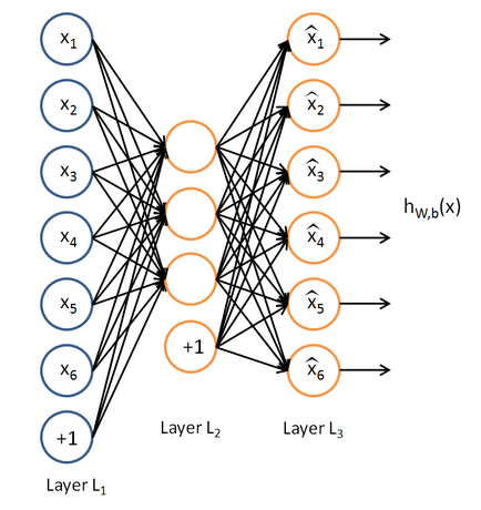
      从图中可以看到，神经网络模型只有一层隐含层，输出层跟输入层的神经单元个数是一样的。如果隐含层单元个数比输入层少的话，我们用这个模型学到的是 输入数据的压缩表示，相当于对输入数据进行降维（这是一种非线性的降维方法）。实际上，如果隐含层单元个数比输入层多，我们可以让隐含层的大部分单元激活值接近0，就是让它们稀疏，这样学到的也是压缩表示。我们模型要使得输出层跟输入层一样，就是隐含层要能够重建出跟输入层一样的输出层，这样我们学到的压缩表示才是有意义的。

     回忆下之前介绍过的损失函数：

   

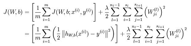
    在这里，y是输出层，跟输入层是一样的。

    自编码神经网络还增加了稀疏性惩罚一项。它是对隐含层进行了稀疏性的约束，即使得隐含层大部分值都处于非active状态。定义隐含层节点j的稀疏程度为

   

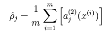
     上式是对整个样本求隐含层节点j的平均值，如果是所有隐含层节点，那么就组成一个向量。

     我们要设置期望隐含层稀疏性的程度，假设为 ，因此我们希望对于所有的节点j 。

     那怎么衡量实际跟期望的差别呢？

     

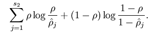
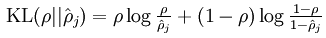      实际上是关于伯努利变量p与q的 KL离散度（参考我之前写的关于信息熵的博客）。

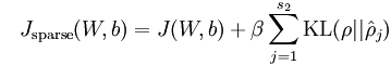
    此时损失函数为

    

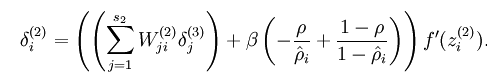
    由于加了稀疏项损失函数，对第二层节点求残差时公式变为

   

实验

       实验教程是在 Exercise:Sparse Autoencoder，要实现的文件是 sampleIMAGES.m, sparseAutoencoderCost.m,computeNumericalGradient.m

     

     实验步骤：

1. 生成训练集
2. 稀疏自编码目标函数
3. 梯度校验
4. 训练稀疏自编码
5. 可视化

       最后一步可视化是 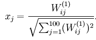，把x用图像表示出来的。

  

      

    代码如下：

sampleIMAGES.m

[plain]  view plain  copy

 

1. <span style="font-size:14px;">function patches = sampleIMAGES()  
2. % sampleIMAGES  
3. % Returns 10000 patches for training  
4.   
5.   
6. load IMAGES;    % load images from disk   
7.   
8.   
9. patchsize = 8;  % we'll use 8x8 patches   
10. numpatches = 10000;  
11.   
12.   
13. % Initialize patches with zeros.  Your code will fill in this matrix--one  
14. % column per patch, 10000 columns.   
15. patches = zeros(patchsize*patchsize, numpatches);  
16.   
17.   
18. %% ---------- YOUR CODE HERE --------------------------------------  
19. %  Instructions: Fill in the variable called "patches" using data   
20. %  from IMAGES.    
21. %    
22. %  IMAGES is a 3D array containing 10 images  
23. %  For instance, IMAGES(:,:,6) is a 512x512 array containing the 6th image,  
24. %  and you can type "imagesc(IMAGES(:,:,6)), colormap gray;" to visualize  
25. %  it. (The contrast on these images look a bit off because they have  
26. %  been preprocessed using using "whitening."  See the lecture notes for  
27. %  more details.) As a second example, IMAGES(21:30,21:30,1) is an image  
28. %  patch corresponding to the pixels in the block (21,21) to (30,30) of  
29. %  Image 1  
30. [m,n,num] = size(IMAGES);  
31.   
32.   
33. for i=1:numpatches  
34.     j = randi(num);  
35.     bx = randi(m-patchsize+1);  
36.     by = randi(n-patchsize+1);  
37.     block = IMAGES(bx:bx+patchsize-1,by:by+patchsize-1,j);  
38.       
39.     patches(:,i) = block(:);  
40. end  
41.   
42.   
43.   
44.   
45.   
46.   
47. %% ---------------------------------------------------------------  
48. % For the autoencoder to work well we need to normalize the data  
49. % Specifically, since the output of the network is bounded between [0,1]  
50. % (due to the sigmoid activation function), we have to make sure   
51. % the range of pixel values is also bounded between [0,1]  
52. patches = normalizeData(patches);  
53.   
54.   
55. end  
56.   
57.   
58.   
59.   
60. %% ---------------------------------------------------------------  
61. function patches = normalizeData(patches)  
62.   
63.   
64. % Squash data to [0.1, 0.9] since we use sigmoid as the activation  
65. % function in the output layer  
66.   
67.   
68. % Remove DC (mean of images).   
69. patches = bsxfun(@minus, patches, mean(patches));  
70.   
71.   
72. % Truncate to +/-3 standard deviations and scale to -1 to 1  
73. pstd = 3 * std(patches(:));  
74. patches = max(min(patches, pstd), -pstd) / pstd;  
75.   
76.   
77. % Rescale from [-1,1] to [0.1,0.9]  
78. patches = (patches + 1) * 0.4 + 0.1;  
79.   
80.   
81. end  
82. </span>  

SparseAutoencoderCost.m

[plain]  view plain  copy

 

1. <span style="font-size:14px;">function [cost,grad] = sparseAutoencoderCost(theta, visibleSize, hiddenSize, ...  
2.                                              lambda, sparsityParam, beta, data)  
3.   
4. % visibleSize: the number of input units (probably 64)   
5. % hiddenSize: the number of hidden units (probably 25)   
6. % lambda: weight decay parameter  
7. % sparsityParam: The desired average activation for the hidden units (denoted in the lecture  
8. %                           notes by the greek alphabet rho, which looks like a lower-case "p").  
9. % beta: weight of sparsity penalty term  
10. % data: Our 64x10000 matrix containing the training data.  So, data(:,i) is the i-th training example.   
11.     
12. % The input theta is a vector (because minFunc expects the parameters to be a vector).   
13. % We first convert theta to the (W1, W2, b1, b2) matrix/vector format, so that this   
14. % follows the notation convention of the lecture notes.   
15.   
16. W1 = reshape(theta(1:hiddenSize*visibleSize), hiddenSize, visibleSize);  
17. W2 = reshape(theta(hiddenSize*visibleSize+1:2*hiddenSize*visibleSize), visibleSize, hiddenSize);  
18. b1 = theta(2*hiddenSize*visibleSize+1:2*hiddenSize*visibleSize+hiddenSize);  
19. b2 = theta(2*hiddenSize*visibleSize+hiddenSize+1:end);  
20.   
21. % Cost and gradient variables (your code needs to compute these values).   
22. % Here, we initialize them to zeros.   
23. cost = 0;  
24. W1grad = zeros(size(W1));   
25. W2grad = zeros(size(W2));  
26. b1grad = zeros(size(b1));   
27. b2grad = zeros(size(b2));  
28.   
29. %% ---------- YOUR CODE HERE --------------------------------------  
30. %  Instructions: Compute the cost/optimization objective J_sparse(W,b) for the Sparse Autoencoder,  
31. %                and the corresponding gradients W1grad, W2grad, b1grad, b2grad.  
32. %  
33. % W1grad, W2grad, b1grad and b2grad should be computed using backpropagation.  
34. % Note that W1grad has the same dimensions as W1, b1grad has the same dimensions  
35. % as b1, etc.  Your code should set W1grad to be the partial derivative of J_sparse(W,b) with  
36. % respect to W1.  I.e., W1grad(i,j) should be the partial derivative of J_sparse(W,b)   
37. % with respect to the input parameter W1(i,j).  Thus, W1grad should be equal to the term   
38. % [(1/m) \Delta W^{(1)} + \lambda W^{(1)}] in the last block of pseudo-code in Section 2.2   
39. % of the lecture notes (and similarly for W2grad, b1grad, b2grad).  
40. %   
41. % Stated differently, if we were using batch gradient descent to optimize the parameters,  
42. % the gradient descent update to W1 would be W1 := W1 - alpha * W1grad, and similarly for W2, b1, b2.   
43. %   
44.   
45. %矩阵向量化形式实现,速度比不用向量快得多  
46. Jcost = 0; %平方误差  
47. Jweight = 0; %规则项惩罚  
48. Jsparse = 0; %稀疏性惩罚  
49. [n, m] = size(data); %m为样本数，这里是10000，n为样本维数，这里是64  
50.   
51. %feedforward前向算法计算隐含层和输出层的每个节点的z值（线性组合值）和a值（激活值）  
52. %data每一列是一个样本，  
53. z2 = W1*data + repmat(b1,1,m); %W1*data的每一列是每个样本的经过权重W1到隐含层的线性组合值,repmat把列向量b1扩充成m列b1组成的矩阵  
54. a2 = sigmoid(z2);  
55. z3 = W2*a2 + repmat(b2,1,m);  
56. a3 = sigmoid(z3);  
57.   
58. %计算预测结果与理想结果的平均误差  
59. Jcost = (0.5/m)*sum(sum((a3-data).^2));  
60. %计算权重惩罚项  
61. Jweight = (1/2)*(sum(sum(W1.^2))+sum(sum(W2.^2)));  
62. %计算稀疏性惩罚项  
63. rho_hat = (1/m)*sum(a2,2);  
64. Jsparse = sum(sparsityParam.*log(sparsityParam./rho_hat)+(1-sparsityParam).*log((1-sparsityParam)./(1-rho_hat)));  
65.   
66. %计算总损失函数  
67. cost = Jcost + lambda*Jweight + beta*Jsparse;  
68.   
69. %反向传播求误差值  
70. delta3 = -(data-a3).*fprime(a3); %每一列是一个样本对应的误差  
71. sterm = beta*(-sparsityParam./rho_hat+(1-sparsityParam)./(1-rho_hat));   
72. delta2 = (W2'*delta3 + repmat(sterm,1,m)).*fprime(a2);  
73.   
74. %计算梯度  
75. W2grad = delta3*a2';  
76. W1grad = delta2*data';  
77. W2grad = W2grad/m + lambda*W2;  
78. W1grad = W1grad/m + lambda*W1;  
79. b2grad = sum(delta3,2)/m; %因为对b的偏导是个向量，这里要把delta3的每一列加起来  
80. b1grad = sum(delta2,2)/m;  
81.   
82. %%----------------------------------  
83. % %对每个样本进行计算, non-vectorial implementation  
84. % [n m] = size(data);  
85. % a2 = zeros(hiddenSize,m);  
86. % a3 = zeros(visibleSize,m);  
87. % Jcost = 0;    %平方误差项  
88. % rho_hat = zeros(hiddenSize,1);   %隐含层每个节点的平均激活度  
89. % Jweight = 0;  %权重衰减项     
90. % Jsparse = 0;   % 稀疏项代价  
91. %   
92. % for i=1:m  
93. %     %feedforward向前转播  
94. %     z2(:,i) = W1*data(:,i)+b1;  
95. %     a2(:,i) = sigmoid(z2(:,i));  
96. %     z3(:,i) = W2*a2(:,i)+b2;  
97. %     a3(:,i) = sigmoid(z3(:,i));  
98. %     Jcost = Jcost+sum((a3(:,i)-data(:,i)).*(a3(:,i)-data(:,i)));  
99. %     rho_hat = rho_hat+a2(:,i);  %累加样本隐含层的激活度  
100. % end  
101. %   
102. % rho_hat = rho_hat/m; %计算平均激活度  
103. % Jsparse = sum(sparsityParam*log(sparsityParam./rho_hat) + (1-sparsityParam)*log((1-sparsityParam)./(1-rho_hat))); %计算稀疏代价  
104. % Jweight = sum(W1(:).*W1(:))+sum(W2(:).*W2(:));%计算权重衰减项  
105. % cost = Jcost/2/m + Jweight/2*lambda + beta*Jsparse; %计算总代价  
106. %   
107. % for i=1:m  
108. %     %backpropogation向后传播  
109. %     delta3 = -(data(:,i)-a3(:,i)).*fprime(a3(:,i));  
110. %     delta2 = (W2'*delta3 +beta*(-sparsityParam./rho_hat+(1-sparsityParam)./(1-rho_hat))).*fprime(a2(:,i));  
111. %   
112. %     W2grad = W2grad + delta3*a2(:,i)';  
113. %     W1grad = W1grad + delta2*data(:,i)';  
114. %     b2grad = b2grad + delta3;  
115. %     b1grad = b1grad + delta2;  
116. % end  
117. % %计算梯度  
118. % W1grad = W1grad/m + lambda*W1;  
119. % W2grad = W2grad/m + lambda*W2;  
120. % b1grad = b1grad/m;  
121. % b2grad = b2grad/m;  
122.   
123. % -------------------------------------------------------------------  
124. % After computing the cost and gradient, we will convert the gradients back  
125. % to a vector format (suitable for minFunc).  Specifically, we will unroll  
126. % your gradient matrices into a vector.  
127. grad = [W1grad(:) ; W2grad(:) ; b1grad(:) ; b2grad(:)];  
128.   
129. end  
130.   
131. %%      Implementation of derivation of f(z)   
132. % f(z) = sigmoid(z) = 1./(1+exp(-z))  
133. % a = 1./(1+exp(-z))  
134. % delta(f) = a.*(1-a)  
135. function dz = fprime(a)  
136.     dz = a.*(1-a);  
137. end  
138. %%  
139. %-------------------------------------------------------------------  
140. % Here's an implementation of the sigmoid function, which you may find useful  
141. % in your computation of the costs and the gradients.  This inputs a (row or  
142. % column) vector (say (z1, z2, z3)) and returns (f(z1), f(z2), f(z3)).   
143.   
144. function sigm = sigmoid(x)  
145.     
146.     sigm = 1 ./ (1 + exp(-x));  
147. end  
148. </span>  

computeNumericalGradient.m

[plain]  view plain  copy

 

1. <span style="font-size:14px;">function numgrad = computeNumericalGradient(J, theta)  
2. % numgrad = computeNumericalGradient(J, theta)  
3. % theta: a vector of parameters  
4. % J: a function that outputs a real-number. Calling y = J(theta) will return the  
5. % function value at theta.   
6.     
7. % Initialize numgrad with zeros  
8. numgrad = zeros(size(theta));  
9.   
10. %% ---------- YOUR CODE HERE --------------------------------------  
11. % Instructions:   
12. % Implement numerical gradient checking, and return the result in numgrad.    
13. % (See Section 2.3 of the lecture notes.)  
14. % You should write code so that numgrad(i) is (the numerical approximation to) the   
15. % partial derivative of J with respect to the i-th input argument, evaluated at theta.    
16. % I.e., numgrad(i) should be the (approximately) the partial derivative of J with   
17. % respect to theta(i).  
18. %                  
19. % Hint: You will probably want to compute the elements of numgrad one at a time.   
20. EPSILON = 1e-4;  
21.   
22. for i=1:length(numgrad)  
23.     theta1 = theta;  
24.     theta1(i) = theta1(i)+EPSILON;  
25.     theta2 = theta;  
26.     theta2(i) = theta2(i)-EPSILON;  
27.       
28.     numgrad(i) = (J(theta1)-J(theta2))/(2*EPSILON);  
29. end  
30.       
31. %% ---------------------------------------------------------------  
32. end  
33. </span>  

如果用向量化计算，几十秒钟就运算出来了，最后结果如下：

   

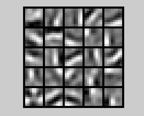
    这里的每幅图像是每个隐含单元的权重表示出来了，每个隐含单元与输入层的所有节点都有权重，令这些权重的2范数为1，把权重表示图像，这样可以大概看出隐含单元总体在学习怎样的一个效果。从图中可以看出不同的隐含单元在学习不同方向和位置的边缘检测，而这个对机器视觉的检测和识别任务是很有帮助的。

在MNIST数据集上实验效果：

实验前要按照 http://ufldl.stanford.edu/wiki/index.php/Exercise:Vectorization上的说明修改参数配置，读入MNIST图像数据，运行10多分钟后的结果如下：

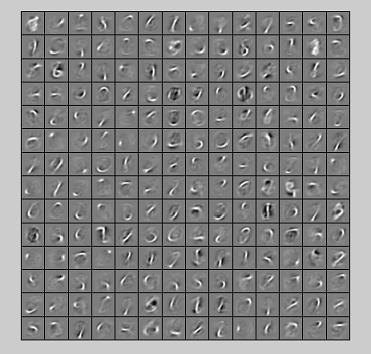
从上面的图看出，这些隐含单元在学习不同数字的笔划边缘。