强化学习——连续控制

前言

本文总结《深度强化学习》中连续控制章节的内容，如有错误，欢迎指出。

连续控制

前面几篇博客总结的强化学习方法，动作空间都是离散有限的。但动作空间不一定总是离散的，也可能是连续的，例如驾驶车辆，汽车转向角度的动作空间就是连续的。针对上述问题，一个可行的解决方案是将动作空间离散化，除此之外，可以直接使用连续控制相关的强化学习方法。本文将总结确定策略梯度算法（DPG）。

DPG

DPG属于策略学习的方法。具体而言，DPG使用Actor-Critic框架，利用价值网络辅助策略网络的训练。DPG的方法框架如下图所示

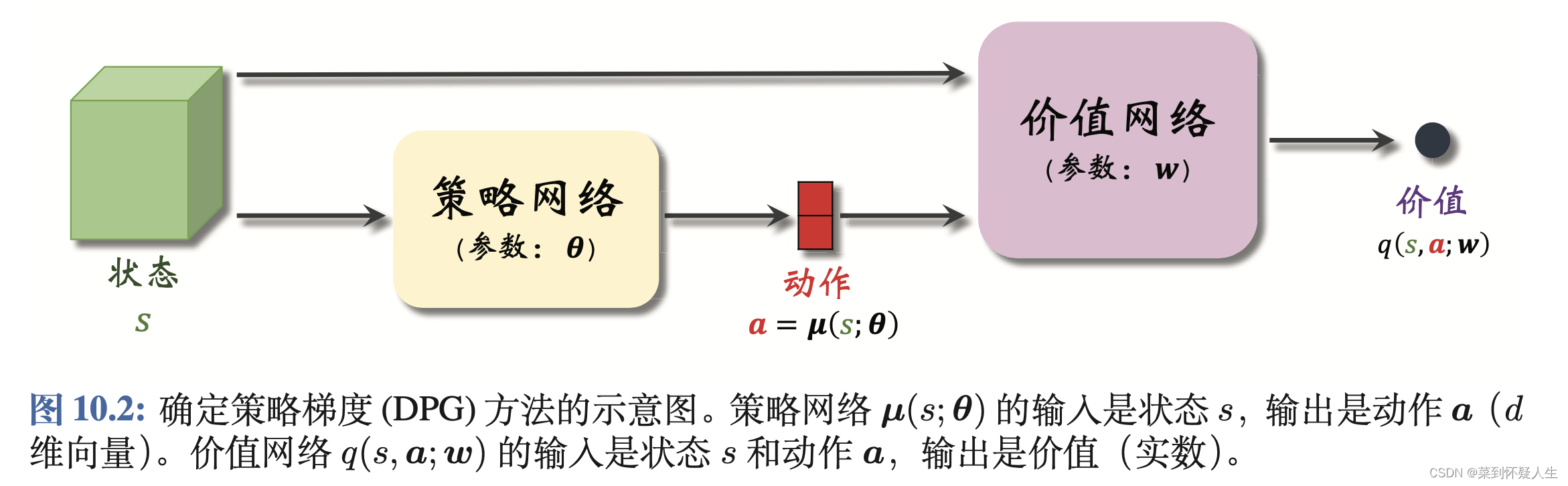
策略网络的输入为状态$s$，输出为智能体执行的具体动作$a=\mu (s;\theta )$。前文介绍的方法，策略网络的输出为智能体执行各个动作的概率，而DPG的输出为一个确定值。将状态$s$与动作$a=\mu (s;\theta )$输入到价值网络中，给出动作的得分$q(s,a;\theta )$。

DPG的优化目标

DPG的优化目标为
$$\max J(\theta )=\max E_S[q(S,\mu (S;\theta );w)]\text{\hspace{1em}(1.0)}$$
$\theta$为策略网络的参数。即希望不论面对什么状态，策略网络的输出都能使价值网络给出较高的分数。因此可得式1.0的梯度为

$${\nabla }_{\theta }J(\theta )=E_S[{\nabla }_{\theta }\mu (S;\theta ){\nabla }_{\theta }q(S,\mu (S;\theta );w)]\text{\hspace{1em}(1.1)}$$

值得一提的是，DPG作为策略学习的一类算法，其目标应该是使状态价值函数的取值最大化，而式1.1与强化学习——策略学习章节推导的随机策略梯度${\nabla }_{\theta }{J}^{\prime }(\theta )$不同，${\nabla }_{\theta }{J}^{\prime }(\theta )$的数学表达式为
$${\nabla }_{\theta }{J}^{\prime }(\theta )=E_S[E_{A\sim \pi (.|S;\theta )}[Q_{\pi }(S,A){\nabla }_{\theta }\ln \pi (A|S;\theta )]]\text{\hspace{1em}(1.2)}$$
设确定策略$\mu (S;\theta )$的输出为$d$维向量，它的第$i$个元素记作${\mu }_i$。设随机策略输出的概率分布为
$$\pi (a|s;\theta ,\delta )=\prod _{i=1}^d\frac{1}{\sqrt{6.28}\delta }\exp (-\frac{[a_i-{\mu }_i]}{2{\delta }_i^2})$$

当$\delta =[{\delta }_1、{\delta }_2、...、{\delta }_d]$为零向量时，存在（具体证明见DPG的论文《Deterministic Policy Gradient Algorithms》）
$$\underset{\delta \to 0}{\lim }{\nabla }_{\theta }{J}^{\prime }(\theta )={\nabla }_{\theta }J(\theta )$$
即确定策略梯度（式1.1）为随机策略梯度（式1.2）的一个特例，优化式子1.1也能使得状态价值函数的取值最大化。

On-Policy DPG

On-Policy DPG(同策略DPG)使用Actor-Critic框架训练策略网络与价值网络，其具体步骤为

• 观测到当前的状态$s_t$，将该状态输入到策略网络中，得到智能体的动作$\mu (s_t;\theta )$。智能体执行该动作后得到新的状态$s_{t+1}$和奖励$r_t$。将状态$s_{t+1}$输入到策略网络中，得到智能体执行的动作$\mu (s_{t+1};\theta )$。
• 计算${\hat{q}}_t=q_{\pi }(s_t,\mu (s_t;\theta );w_{now})$、${\hat{q}}_{t+1}=q_{\pi }(s_{t+1},\mu (s_{t+1};\theta );w_{now})$
• 利用贝尔曼方程优化价值网络$q(s,a;w)$ $$w_{new}=w_{now}-\alpha [{\hat{q}}_t-(r_t+{\hat{q}}_{t+1})]{\nabla }_{w}q(s_t,\mu (s_t;\theta );w_{now})$$
• 更新策略网络$${\theta }_{new}={\theta }_{now}+\beta {\nabla }_{\theta }{\hat{q}}_t{\nabla }_{\theta }\mu (s_t;\theta )$$

Off-Policy DPG

DPG的策略网络输出的动作是确定的，因此同策略DPG难以充分探索环境，网络可能收敛至局部最小值。值得一提的是，随机策略梯度的策略网络输出的动作是概率分布，依据概率采样动作（概率小的动作也可能被采样）可以让智能体充分探索环境。

异策略DPG（Off-Policy DPG）解决同策略DPG难以充分探索环境的问题。值得一提的是，同策略DPG的价值网络拟合的是动作价值函数，而异策略DPG的价值网络拟合的是最优动作价值函数。同策略DPG使用SARSA算法训练价值网络，而异策略DPG使用Q-learning训练价值网络。

异策略DPG训练策略网络和价值网络的流程为

• 开始训练前，利用策略网络控制智能体在环境中运动，得到一系列的四元组($s_t,a_t,s_{t+1},a_{t+1}$)，所有的四元组构成经验回放数组
• 从经验回放数组中抽取四元组($s_t,a_t,s_{t+1},a_{t+1}$)，通过策略网络计算
  $${\hat{a}}_t=\mu (s_t;{\theta }_{now}){\hat{a}}_{t+1}=\mu (s_{t+1};{\theta }_{now})$$
• 利用价值网络计算（注意动作的符号）
  $${\hat{q}}_t=q(s_t,a_t;w_{now}){\hat{q}}_{t+1}=q(s_{t+1},{\hat{a}}_{t+1};w_{now})$$
• 更新价值网络的参数
  $$w_{new}=w_{now}-\alpha [{\hat{q}}_t-(r_t+{\hat{q}}_{t+1})]{\nabla }_{w}q(s_t,\mu (s_t;\theta );w_{now})$$
• 更新策略网络的参数
  $${\theta }_{new}={\theta }_{now}+\beta {\nabla }_{\theta }q(s_t,{\hat{a}}_t;w){\nabla }_{\theta }\mu (s_t;{\theta }_{now})$$

值得一提的是，异策略DPG让价值网络拟合最优动作价值函数$Q_{\ast }(s,a;\theta )$，因此其希望策略网络输出的动作为
$$\mu (s;\theta )\approx \underset{a}{\mathrm{argmax}}{Q}_{\ast }(s,a;\theta )$$
由于异策略DPG的价值网络使用最优贝尔曼方程进行优化，因此其存在最大化、自举导致的高估问题（可以浏览强化学习——价值学习中的DQN章节）。对于此类问题，可以使用Twin Delayed Deep Deterministic Policy Gradient（TD3）解决。TD3含有两个价值网络，两个目标价值网络，一个策略网络，一个目标策略，其具体训练流程为

• 初始阶段，随机初始化两个目标网络的参数$w_1、w_2$以及策略网络的参数$\theta$。接着初始化两个目标价值网络的参数$w_1^{-}、w_2^{-}$以及目标策略网络的参数${\theta }^{-}$为
  $$\begin{gathered} w_1^{-}=w_1 \\ {w}_2^{-}=w_2 \\ {\theta }^{-}=\theta \end{gathered}$$

• 开始训练前，利用某种策略控制智能体与环境交互，获得一系列四元组($s_t,a_t,r_t,s_{t+1}$)，这些四元组成经验回放数组。

• 训练时，从经验回放数组中抽取一个四元组($s_t,a_t,r_t,s_{t+1}$)，让目标策略网络计算
  $${\hat{a}}_{j+1}^{-}=\mu (s_{j+1};{\theta }_{now}^{-})+ϵ$$其中$ϵ$为截断独立正态分布中抽取的随机噪声，这个步骤视为了缓解最大化导致的高估问题

• 让两个目标价值网络预测，这一步骤用于缓解自举导致的高估问题
  $$\begin{array}{rl}{\hat{q}}_{1,j+1}^{-}& =q(s_{j+1},{\hat{a}}_{j+1}^{-};w_{1,now}^{-})\\ {\hat{q}}_{2,j+1}^{-}& =q(s_{j+1},{\hat{a}}_{j+1}^{-};w_{2,now}^{-})\end{array}$$

• 计算TD误差 y ^ j = r j + min ⁡ { q ^ 1 , j + 1 − , q ^ 2 , j + 1 − } \hat y_j=r_j+\min\{\hat q_{1,j+1}^-,\hat q_{2,j+1}^-\} y^​j​=rj​+min{q^​1,j+1−​,q^​2,j+1−​}

• 更新两个价值网络
  $$\begin{array}{rl}{w}_{1,new}& =w_{1,now}-\alpha ({\hat{q}}_{1,j+1}^{-}-{\hat{y}}_j){\nabla }_{w_1}q(s_j,a_j;w_{1,now})\\ w_{2,new}& =w_{2,now}-\alpha ({\hat{q}}_{2,j+1}^{-}-{\hat{y}}_j){\nabla }_{w_2}q(s_j,a_j;w_{2,now})\end{array}$$

• 每隔k轮更新一次策略网络和三个目标网络

  • 让策略网络计算${\hat{a}}_t=\mu (s_t;{\theta }_{now})$，接着更新策略网络$${\theta }_{new}={\theta }_{now}+\beta {\nabla }_{\theta }q(s_t,{\hat{a}}_t;w){\nabla }_{\theta }\mu (s_t;{\theta }_{now})$$
  • 用动量方式更新三个策略网络参数，$\gamma$为超参数
    $$\begin{array}{rl}{\theta }_{new}^{-}& =\gamma {\theta }_{new}+(1-\gamma ){\theta }_{now}^{-}\\ w_{1,new}^{-}& =\gamma w_{1,new}+(1-\gamma )w_{1,now}^{-}\\ w_{2,new}^{-}& =\gamma w_{2,new}+(1-\gamma )w_{2,now}^{-}\end{array}$$

随机高斯策略

除去使用DPG解决连续控制问题外，还可以使用随机高斯策略解决。随机高斯策略假设策略函数服从高斯分布：
$$\pi (a|s;\theta ,\delta )=\prod _{i=1}^d\frac{1}{\sqrt{6.28}\delta }\exp (-\frac{[a_i-{\mu }_i]}{2{\delta }_i^2})$$

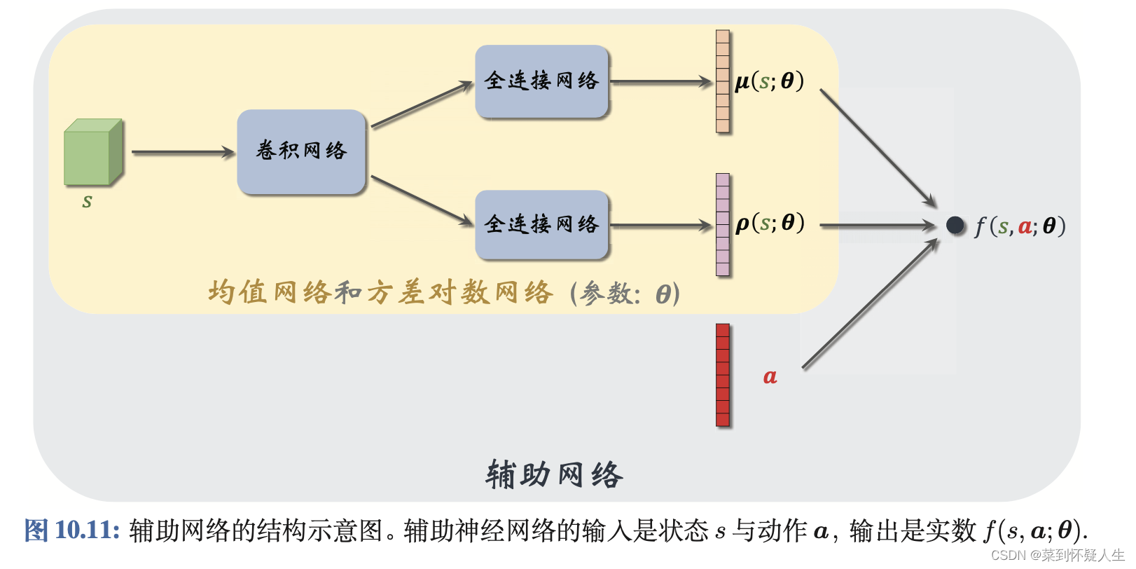
其使用两个神经网络$\mu (s;\theta )$、$\rho (s;\theta )$拟合高斯分布的均值$\mu$和对数方差$\ln \delta$，均值和方差神经网络（又称为辅助网络）的结构图为

随机高斯策略的训练流程为

• 观测到当前的状态$s_t$，计算均值、方差$\mu (s_t;\theta )$、$\exp (\rho (s_t;\theta ))$，从高斯分布中采样动作$a$
• 计算动作价值函数$Q_{\pi }(s,a)$
• 用反向传播计算辅助网络关于参数$\theta$的梯度$${\nabla }_{\theta }\ln \pi (a|s;\theta )$$
• 计算策略梯度
  $$Q_{\pi }(s,a){\nabla }_{\theta }\ln \pi (a|s;\theta )$$
• 用梯度上升法更新辅助网络的参数
  $${\theta }_{new}={\theta }_{now}+\beta Q_{\pi }(s,a){\nabla }_{\theta }\ln \pi (a|s;\theta )$$

上述训练流程中的$Q_{\pi }(s,a)$可以使用策略学习中的REINFORCE方法或Actor-Critic方法近似，具体查阅强化学习——策略学习。

测试时，将状态$S$输入到卷积神经网络中，卷积神经网络的输出经过两个并行的全连接网络，得到高斯分布的均值和对数方差$\mu (s;\theta )$、$\rho (s;\theta )$，接着从高斯分布中采样得到智能体执行的动作。