数学基础

 

线性代数：

n维向量x乘以x的转置就是一个对称矩阵

矩阵转置时主对角的元素不变 

矩阵乘法的计算规则如下图：

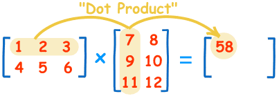
为什么是这样的计算规则，参考：Linear Algebra: What matrices actually are

Most high school students in the United States learn about matrices and matrix multiplication, but they often are not taught why matrix multiplication works the way it does. Adding matrices is easy: you just add the corresponding entries. However, matrix multiplication does not work this way, and for someone who doesn’t understand the theory behind matrices, this way of multiplying matrices may seem extremely contrived and strange. To truly understand matrices, we view them as representations of part of a bigger picture. Matrices represent functions between spaces, called vector spaces, and not just any functions either, but linear functions. This is in fact why linear algebra focuses on matrices. The two fundamental facts about matrices is that every matrix represents some linear function, and every linear function is represented by a matrix. Therefore, there is in fact a one-to-one correspondence between matrices and linear functions. We’ll show that multiplying matrices corresponds to composing the functions that they represent. Along the way, we’ll examine what matrices are good for and why linear algebra sprang up in the first place.

 

Most likely, if you’ve taken algebra in high school, you’ve seen something like the following:

Your high school algebra teacher probably told you this thing was a “matrix.”  You then learned how to do things with matrices. For example, you can add two matrices, and the operation is fairly intuitive:

You can also subtract matrices, which works similarly. You can multiply a matrix by a number:

Then, when you were taught how to multiply matrices, everything seemed wrong:

That is, to find the entry in the -th row, -th column of the product, you look at the -th row of the first matrix, the -th column of the second matrix, you multiply together their corresponding numbers, and then you add up the results to get the entry in that position. In the above example, the 1st row, 2nd column entry is a  because the 1st row of the first matrix is , the 2nd column of the second matrix is , and we have . Moreover, this implies that matrix multiplication isn’t even commutative! If we switch the order of multiplication above, we get

How come matrix multiplication doesn’t work like addition and subtraction? And if multiplication works this way, how the heck does division work? The goal of this post is to answer these questions.

To understand why matrix multiplication works this way, it’s necessary to understand what matrices actually are. But before we get to that, let’s briefly take a look at why we care about matrices in the first place. The most basic application of matrices is solving systems of linear equations. A linear equation is one in which all the variables appear by themselves with no powers; they don’t get multiplied with each other or themselves, and no funny functions either. An example of a system of linear equations is

The solution to this system is . Such equations seem simple, but they easily arise in life. For example, let’s say I have two friends Alice and Bob who went shopping for candy. Alice bought 2 chocolate bars and 1 bag of skittles and spent $3, whereas Bob bought 4 chocolate bars and 3 bags of skittles and spent $7. If we want to figure out how much chocolate bars and skittles cost, we can let  be the price of a chocolate bar and  be the price of a bag of skittles and the variables would satisfy the above system of linear equations. Therefore we can deduce that a chocolate bar costs $1 and so does a bag of skittles. This system was particularly easy to solve because one can guess and check the solution, but in general, with  variables and equations instead of 2, it’s much harder. That’s where matrices come in! Note that, by matrix multiplication, the above system of linear equations can be re-written as

If only we could find a matrix , which is the inverse of the matrix , so that if we multiplied both sides of the equation (on the left) by  we’d get

The applications of matrices reach far beyond this simple problem, but for now we’ll use this as our motivation. Let’s get back to understanding what matrices are. To understand matrices, we have to know what vectors are. A vector space is a set with a specific structure, and a vector is simply an element of the vector space. For now, for technical simplicity, we’ll stick with vector spaces over the real numbers, also known as real vector spaces. A real vector space is basically what you think of when you think of space. The number line is a 1-dimensional real vector space, the x-y plane is a 2-dimensional real vector space, 3-dimensional space is a 3-dimensional real vector space, and so on. If you learned about vectors in school, then you are probably familiar with thinking about them as arrows which you can add together, multiply by a real number, and so on, but multiplying vectors together works differently. Does this sound familiar? It should. That’s how matrices work, and it’s no coincidence.

The most important fact about vector spaces is that they always have a basis. A basis of a vector space is a set of vectors such that any vector in the space can be written as a linear combination of those basis vectors. If  are your basis vectors, then  is a linear combination if  are real numbers. A concrete example is the following: a basis for the x-y plane is the vectors . Any vector is of the form  which can be written as

so we indeed have a basis! This is not the only possible basis. In fact, the vectors in our basis don’t even have to be perpendicular! For example, the vectors  form a basis since we can write

.

Now, a linear transformation is simply a function between two vector spaces that happens to be linear. Being linear is an extremely nice property. A function  is linear if the following two properties hold:

For example, the function  defined on the real line is not linear, since  whereas . Now, we connect together all the ideas we’ve talked about so far: matrices, basis, and linear transformations. The connection is that matrices are representations of linear transformations, and you can figure out how to write the matrix down by seeing how it acts on a basis. To understand the first statement, we need to see why the second is true. The idea is that any vector is a linear combination of basis vectors, so you only need to know how the linear transformation affects each basis vector. This is because, since the function is linear, if we have an arbitrary vector  which can be written as a linear combination , then

Notice that the value of  is completely determined by the values , and so that’s all the information we need to completely define the linear transformation. Where does the matrix come in? Well, once we choose a basis for both the domain and the target of the linear transformation, the columns of the matrix will represent the images of the basis vectors under the function. For example, suppose we have a linear transformation  which maps  to , meaning it takes in 3-dimensional vectors and spits out 2-dimensional vectors. Right now  is just some abstract function for which we have no way of writing down on paper. Let’s pick a basis for both our domain (3-space) and our target (2-space, or the plane). A nice choice would be  for the former and  for the latter. All we need to know is how  affects , and the basis for the target is for writing down the values  concretely. The matrix  for our function will be a 2-by-3 matrix, where the 3 columns are indexed by  and the 2 rows are indexed by . All we need to write down  are the values . For concreteness, let’s say

Then the corresponding matrix will be

The reason why this works is that matrix multiplication was designed so that if you multiply a matrix by the vector with all zeroes except a 1 in the -th entry, then the result is just the -th column of the matrix. You can check this for yourself. So we know that the matrix  works correctly when applied to (multiplied to) basis vectors. But also matrices satisfy the same properties as linear transformations, namely  and , where  are vectors and  is a real number. Therefore  works for all vectors, so it’s the correct representation of . Note that if we had chosen different vectors for the basis vectors, the matrix would look different. Therefore, matrices are not natural in the sense that they depend on what bases we choose.

Now, finally to answer the question posed at the beginning. Why does matrix multiplication work the way it does? Let’s take a look at the two matrices we had in the beginning:  and . We know that these correspond to linear functions on the plane, let’s call them  and , respectively. Multiplying matrices corresponds to composing their functions. Therefore, doing  is the same as doing  for any vector . To determine what the matrix  should look like, we can see how it affects the basis vectors . We have

so the first column of  should be , and

so the second column of  should be . Indeed, this agrees with the answer we got in the beginning by matrix multiplication! Although this is not at all a rigorous proof, since it’s just an example, it captures the idea of the reason matrix multiplication is the way it is.

Now that we understand how and why matrix multiplication works the way it does, how does matrix division work? You are probably familiar with functional inverses. The inverse of a function  is a function  such that  for all . Since multiplication of matrices corresponds to composition of functions, it only makes sense that the multiplicative inverse of a matrix is the compositional inverse of the corresponding function. That’s why not all matrices have multiplicative inverses. Some functions don’t have compositional inverses! For example, the linear function  mapping  to  defined by  has no inverse, since many vectors get mapped to the same value (what would  be? ? ?). This corresponds to the fact that the 1×2 matrix  has no multiplicative inverse. So dividing by a matrix  is just multiplication by , if it exists. There are algorithms for computing inverses of matrices, but we’ll save that for another post.

 

 

（1）你有感觉到某一类矩阵和矩阵相乘，其实就是解方程时的消元吗？

（2）

你有发现解方程时对矩阵的操作，与消元法解方程的对应关系吗？

你有发现行列式的定义和性质，与消元法解方程的对应关系吗？

你有发现求逆矩阵与消元法解方程的对应关系吗？而奇异矩阵与这个消元法解方程又有什么关系呢？

你有发现非常自然的消元法解方程，是连结矩阵、行列式、逆矩阵这些概念线索和纽带吗？这么普普通通的消元法解方程是多少线性代数基础概念的核心啊！所有的东西都不是无中生有的，

线性代数的设定真的不是像国内那些垃圾教材里面描述的好像一只孙猴子一样，像直接从石头缝里蹦出来的啊！

（3）前面已经提到了，三种“理解矩阵变换”，你理解了吗？

（4）为什么行秩和列秩是一样的？涉及四个基本子空间（列空间，零空间，行空间，左零空间），这个东西是我最近才感悟到的。

 

 

 

概率统计：

（1）极大似然思想

（2）贝叶斯模型

（3）隐变量混合概率模型，EM思想

（4）基础的典型分布如高斯分布

 

微积分：

（1）极值问题 与 （条件）最优化问题

（2）偏导数，梯度

（3）凸优化和条件最优化问题，这个是理解SVM，或者线性回归等等模型正则化的基础

 

 

 

公开课与相关文献：

 

（1）麻省理工公开课：线性代数   http://open.163.com/special/opencourse/daishu.html

（2）斯坦福大学公开课 ：机器学习课程   http://open.163.com/special/opencourse/machinelearning.html

（3）知乎 https://www.zhihu.com/question/36324957

（4）凸优化 http://www.bilibili.com/video/av8907218/

 

 

 

 

 

转载于:https://www.cnblogs.com/mazhimazhi/p/7816610.html